REVIEW 4 major objections 7 minor 42 references
Spectral Learning of Magnetized Plasma Dynamics: A Neural Operator Application
T0 review · 4 major / 7 minor · reviewed 2026-08-06 · deepseek-v4-flash
Pith's one-line read A machine-learning operator trained on short simulation windows can forecast 2D magnetized turbulence for parameter values it never saw.
desk verdict A solid short-horizon FNO benchmark for the Orszag-Tang vortex, but the long-horizon and 96% accuracy claims outrun what is actually quantified. read the letter →
The pith
A machine-rendered reading of the paper's core claim, the machinery that carries it, and where it could break.
The reading
What carries the argument
The central object is the Fourier neural operator, an architecture that replaces the integral kernel of a neural operator with a convolution performed in Fourier space: transform the input, multiply by a learned weight tensor, truncate high modes, transform back, and combine with a local convolution. Here it is configured with five Fourier layers of width 30, 64 Fourier modes, and a block-based forecasting scheme (five input frames spaced 20 steps, ten output frames spaced 80 steps, iterated as blocks) so the operator maps a short history plus physical parameters to a future window. The mode truncation is what gives the model its speed and also its blindness to the smallest resolved scales.
What would settle it
A concrete test: run the trained model autoregressively for the full 640-frame window on a held-out parameter set and plot block-wise MSE against the solver at each frame; if the MSE at $t = 4\,t_A$ exceeds the single-block value by roughly an order of magnitude, or if the predicted power spectrum diverges from the target at intermediate wavenumbers, the long-coherence claim is falsified.
Extended reading notes
Core claim
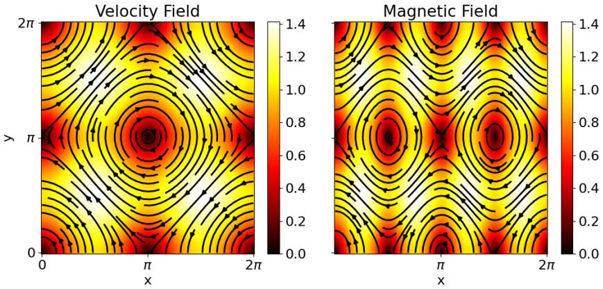
On the paper's own terms, the discovery is that a five-layer Fourier neural operator with 64 retained Fourier modes, fed five snapshots plus the viscosity and diffusivity, can output ten future snapshots and be chained blockwise to forecast the Orszag-Tang vortex over hundreds of timesteps. For held-out viscosity and diffusivity values the mean-squared error is about $6 \times 10^{-3}$ in velocity and about $10^{-3}$ in magnetic field; power spectra and dissipation rates match the solver to about 96%. The model captures large- and intermediate-scale structures and degrades at small scales, where Fourier-mode truncation removes the dissipative range. Against a UNet baseline it reduces error by 97%, and at inference it is about 25x faster than a GPU-oriented high-order finite-volume solver. The authors frame this as evidence that FNOs can serve as accurate surrogates for magnetized turbulence across the sampled parameter range.
Load-bearing premise
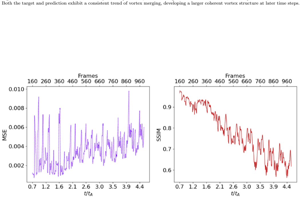
The long-horizon prediction claim rests on the assumption that chaining the five-to-ten-frame blocks produces temporally coherent forecasts without unbounded error growth; the authors themselves report that MSE rises over time and that later channels in each block are under-weighted, so stability across blocks is assumed rather than demonstrated.
Editorial extensions
If this is right
- The trained model can replace roughly 80% of a solver run, so a full simulation becomes a short solver burst followed by neural continuation.
- Parameter sweeps in viscosity and diffusivity that previously required many solver runs can be emulated at about 25x inference speed, making dissipation studies over the parameter plane practical.
- The architecture generalizes to unseen parameter combinations within the trained range, so the surrogate does not need retraining for every new viscosity and diffusivity pair.
- Spectral fidelity holds at large and intermediate wavenumbers, meaning derived quantities like energy spectra and dissipation rates remain reliable even where pointwise fields carry small-scale errors.
- Performance degrades on coarser grids and fewer modes, so the method's usable range is bounded by spatial resolution and by the number of Fourier modes retained.
Reading between the lines
- The paper's own discussion notes that error grows over time and that the model prioritizes early input channels; a natural testable extension is to randomize frame offsets or apply mirroring during training to break that channel bias and improve chaining stability.
- Because the small-scale bottleneck is tied to mode truncation, applying the same blockwise scheme to other periodic MHD benchmarks will likely hit the same wall at shocks and current sheets; adding adaptive or extra modes near discontinuities is a concrete direction the paper does not explore.
- If blockwise chaining can be made stable, FNO surrogates of this kind could be embedded in Bayesian parameter estimation or data assimilation for astrophysical plasmas, where many forward evaluations are needed.
- The reported 96% accuracy on dissipation suggests the surrogate could cheaply map the viscosity-diffusivity plane of dissipation diagnostics, though the paper itself does not perform such a sweep.
Editorial analysis
A structured set of objections, weighed in public.
Referee Report
Summary. The manuscript presents a Fourier neural operator (FNO) surrogate trained on FARGO3D simulations of the 2D Orszag-Tang vortex for a range of viscosities and magnetic diffusivities. The model maps blocks of five input frames at one cadence to ten output frames at another cadence, and is evaluated on held-out parameter pairs. The authors report MSE values at t=1 tA, a baseline comparison with a UNet, spectral and dissipation-rate comparisons, and an inference speed-up of about 25x. The central claims are that the FNO generalizes to unseen parameters, reproduces energy spectra and dissipation rates within 96% accuracy, and retains temporal coherence over long timescales.
Significance. Neural surrogates for MHD turbulence are of genuine interest, and the Orszag-Tang vortex is a good choice of benchmark. The paper's strengths are that the ground truth comes from a well-established external solver (FARGO3D), the test parameters are held out from training, a UNet baseline is included on equal footing, and the speed-up measurement is performed on the same hardware. If the quantitative claims (MSE ~6e-3/1e-3, 96% spectral/dissipation accuracy, 97% error reduction over UNet, temporal coherence over long timescales) were backed by the reported metrics, this would be a useful contribution to the neural-operator literature for plasma physics. At present, however, these headline numbers are not derivable from the tables and figures shown, so the significance of the contribution is not yet established.
major comments (4)
- [Abstract; §5.3–5.4; §5.7] The abstract states that the model 'reproduces energy spectra and dissipation rates within 96% accuracy' and 'cuts error by 97%' relative to a UNet baseline, but no equation, table, or figure quantifies either number. Figures 14–18 are qualitative comparisons of dissipation and power spectra, and Figure 22 shows MSE curves without reporting the numerical values used to compute a 97% reduction. The authors should define the accuracy metric (e.g., relative L2 error of P(k) and ε(t)), report the computed values for the held-out cases, and provide the actual MSE numbers behind the UNet comparison. Without this, the headline quantitative claims are not verifiable.
- [§3.4, §4.2, §6, Figs. 9/13, Appendix B] The claim that the model 'retains temporal coherence over long timescales' is not supported by any long-horizon metric. The only tabulated errors (Table 1) are at t=1 tA; Figures 9 and 13 show MSE increasing and SSIM decreasing over time; and Section 6 states that 'the model tends to prioritize the initial channels' and that there is 'reduced accuracy at the end of each block.' Appendix B (e.g., Figures B.25 and B.28) shows the time dependence of MSE but does not report a cumulative rollout error either. The authors should report per-block and cumulative MSE/SSIM over the full 0.73–4.39 tA interval, ideally comparing chained autoregressive predictions with one-shot predictions, and quantify the error growth rate.
- [§4.1, §5.1–5.2, Conclusions (iii)] The generalization claim for unseen parameters rests on a single main-text test case (ν=µ=5×10^-5). The two additional test cases in Appendix B are run at 64×64 resolution with only 8 Fourier modes, so they do not test the main 128×128, 64-mode configuration; moreover, they visibly degrade at later times. No error bars or multiple training seeds are provided anywhere, and the hyperparameter selection process (Section 3.4) does not state which data were used for model selection. To support the generalization conclusion, the authors should report metrics for all held-out parameter pairs at the main configuration, with statistics over at least three seeds, and describe the hyperparameter tuning protocol.
- [§3.4, §4.2] The iterative block-forecasting algorithm is under-specified. The text gives input/output block sizes and cadences, but does not describe how consecutive blocks are chained (e.g., whether the last five predicted frames become the input to the next block, how the physical parameters (ν, η) are appended per block, and how the 5 input frames 'spaced t=1.0 code units apart' relate to the 'timestep of 20' mentioned in Section 6). Without a precise algorithm, the long-term rollout is not reproducible, and the claimed 80% acceleration cannot be independently assessed. Please provide a step-by-step pseudocode or diagram of the chaining process.
minor comments (7)
- [Abstract vs. §3.1] The abstract calls FARGO3D a 'high-order finite-volume solver', but Section 3.1 says it 'employs the finite-difference method'; please reconcile.
- [Throughout] The magnetic diffusivity is denoted η in the abstract and induction equation but µ in Eqs. (24)–(25) and in parts of the text; use one symbol consistently.
- [§2, Eq. (4)] Equation (4) omits the viscous and Ohmic heating terms in the energy equation; as written it is not the full nonideal MHD energy equation. Please state that the FARGO3D simulations use the full equations and that Eq. (4) is a simplified form.
- [Language] The typographical errors should be corrected (e.g., 'rennasaince', 'archictetures', 'numers', 'dicuss', 'nd diffusivity', 'nondeal', 'matrice').
- [§2, references] The characterization of Orszag & Tang (1979) as a parametric study of viscosity and diffusivity appears inaccurate; that paper studies small-scale structure of 2D MHD turbulence for fixed parameters. Please revise or cite a more appropriate reference.
- [Supplementary Materials] The statement that code and data 'will be made available soon' is not sufficient for reproducibility; please provide a link or an explicit reason for the delay.
- [§5.6] Please clarify that the 25× speed-up is inference-only and does not include the training cost, and specify whether the timing includes I/O and data preprocessing for the FARGO3D run.
Circularity Check
No meaningful circularity: the prediction claims are validated against held-out FARGO3D simulations, an external numerical solver, and the only self-citation is a non-load-bearing UNet baseline reference.
full rationale
The central claims of the paper are empirical: the reported MSE values, power-spectrum comparisons, dissipation-rate tracking, and speed-up are all evaluated against FARGO3D ground-truth data rather than derived from the training objective itself. Generalization is tested on parameter pairs explicitly held out from training (Section 4.1 reserves nu=mu=5e-5 and nu=mu=3e-4 for evaluation), so the 'unseen parameter settings' claim is not a restatement of the fitted training loss. The FNO architecture is adopted from the external prior work of Li et al. (2021), and the numerical solver is the independent FARGO3D code, so no load-bearing result is imported from the present authors' own prior papers. The only self-citation is Duarte, Nemmen and Navarro (2022), used in Section 5.7 solely to specify the UNet baseline implementation; this does not support any central claim of the paper. The manuscript's own Discussion (Section 6) explicitly concedes that block-based forecasting loses accuracy at the end of each block and that 'the model tends to prioritize the initial channels,' which is an honest limitation of the long-horizon claim rather than a circular step. Likewise, the abstract's '96% accuracy' for energy spectra and dissipation rates is not accompanied by a defined error metric, and no end-of-rollout error is tabulated; these are reporting gaps concerning correctness and robustness, not self-referential derivations. No equation or fitted parameter is renamed as a prediction, and no uniqueness argument or ansatz is smuggled in via self-citation. Accordingly, there is no circular step that reduces the paper's results to its inputs by construction.
Assumptions & free parameters
free parameters (3)
- Fourier mode truncation =
64 spatial modes, 5 temporal modes
- Temporal block sizes =
input 5 frames (cadence 20 steps), output 10 frames (cadence 80 steps)
- Hyperparameters (layers, width, learning rate) =
5 Fourier layers, width 30, Adam LR=0.001
assumptions (4)
- domain assumption The 2D non-ideal MHD equations (Eqs. 1-4) with the given initial conditions are an accurate model of the Orszag-Tang vortex.
- domain assumption FARGO3D's finite-difference with constrained transport yields converged solutions at 128x128 for the lowest dissipation cases.
- ad hoc to paper The global min-max normalization (Eq. 26) computed over the training set remains valid for test parameters.
- ad hoc to paper The autoregressive block prediction scheme yields bounded error growth over long horizons.
Cite this review
Pith. "Pith review of Spectral Learning of Magnetized Plasma Dynamics: A Neural Operator Application." pith.science (2026). https://pith.science/paper/LLLNTI74
@misc{pith2026250701388,
  author       = {Pith},
  title        = {Pith review of: Spectral Learning of Magnetized Plasma Dynamics: A Neural Operator Application},
  year         = {2026},
  howpublished = {\url{https://pith.science/paper/LLLNTI74}},
  note         = {Machine review of arXiv:2507.01388}
}
abstract
Fourier neural operators (FNOs) provide a mesh-independent way to learn solution operators for partial differential equations, yet their efficacy for magnetized turbulence is largely unexplored. Here we train an FNO surrogate for the 2-D Orszag-Tang vortex, a canonical non-ideal magnetohydrodynamic (MHD) benchmark, across an ensemble of viscosities and magnetic diffusivities. On unseen parameter settings the model achieves a mean-squared error of $\approx 6 \times 10^{-3}$ in velocity and $\approx 10^{-3}$ in magnetic field, reproduces energy spectra and dissipation rates within $96\%$ accuracy, and retains temporal coherence over long timescales. Spectral analysis shows accurate recovery of large- and intermediate-scale structures, with degradation at the smallest resolved scales due to Fourier-mode truncation. Relative to a UNet baseline the FNO cuts error by $97\%$, and compared with a high-order finite-volume solver it delivers a $25\times$ inference speed-up, offering a practical path to rapid parameter sweeps in MHD simulations.
Figures


Figures from the paper (20 more)




Reference graph
Works this paper leans on
-
[1]
M. Cranmer, S. Greydanus, S. Hoyer, P. Battaglia, D. Spergel, and S. Ho, “Lagrangian neural networks,” in International Conference on Learning Representations, (Online Conference), 2020
work page 2020
-
[2]
S.Greydanus, M.Dzamba, andJ.Yosinski, “Hamiltonianneural networks,” inNeural Information Processing Systems, (Vancou- ver, Canada), 2019. 23 Figure B.28: MSE over time between predictions and ground truth for|u| and |B| for the caseν = 3 × 10⁻⁴ and µ = 10−4. Figure C.29: Temporal evolution of theux velocity component from t = 1 to t = 4 t/tA. The plot sho...
work page 2019
-
[3]
Learning Mesh-Based Simulation with Graph Net- works,
T. Pfaff, M. Fortunato, A. Sanchez-Gonzalez, and P. W. Battaglia, “Learning Mesh-Based Simulation with Graph Net- works,” in Neural Information Processing Systems, (Online Conference), 2020
work page 2020
-
[4]
J. Pathak, A. Wikner, R. Fussell, S. Chandra, B. R. Hunt, M. Girvan, and E. Ott, “Hybrid forecasting of chaotic processes: Using machine learning in conjunction with a knowledge-based model,” Chaos: An Interdisciplinary Journal of Nonlinear Sci- ence, vol. 28, no. 4, p. 041101, 2018
work page 2018
-
[5]
A. Mohan, D. Daniel, M. Chertkov, and D. Livescu, “Com- pressed convolutional lstm: An efficient deep learning frame- work to model high fidelity 3d turbulence,” 2019
work page 2019
-
[6]
Newton versus the machine: solving the chaotic three-body problem using deep neural networks,
P. G. Breen, C. N. Foley, T. Boekholt, and S. Portegies Zwart, “Newton versus the machine: solving the chaotic three-body problem using deep neural networks,” Mon. Not. R. Astron. Soc., vol. 494, pp. 2465–2470, May 2020
work page 2020
-
[7]
Machine learning for fluid mechanics,
S. L. Brunton, B. R. Noack, and P. Koumoutsakos, “Machine learning for fluid mechanics,”Annual Review of Fluid Mechan- ics, vol. 52, no. 1, pp. 477–508, 2020
work page 2020
-
[8]
Convolutional neural networks for steady flow approximation,
X. Guo, W. Li, and F. Iorio, “Convolutional neural networks for steady flow approximation,” inProceedings of the 22nd ACM SIGKDD International Conference on Knowledge Discovery and Data Mining, KDD ’16, (New York, NY, USA), pp. 481– 490, Association for Computing Machinery, 2016
work page 2016
Show all 42 references
-
[9]
Accelerating eulerian fluid simulation with convolutional net- works,
J. Tompson, K. Schlachter, P. Sprechmann, and K. Perlin, “Accelerating eulerian fluid simulation with convolutional net- works,” CoRR, vol. abs/1607.03597, 2016
2016 arXiv
-
[10]
Deep fluids: A generative network for parame- terized fluid simulations,
B. Kim, V. C. Azevedo, N. Thuerey, T. Kim, M. Gross, and B. Solenthaler, “Deep fluids: A generative network for parame- terized fluid simulations,”Computer Graphics Forum, vol. 38, no. 2, pp. 59–70, 2019
2019
-
[11]
Machinelearning–acceleratedcomputational fluid dynamics,
D. Kochkov, J. A. Smith, A. Alieva, Q. Wang, M. P. Bren- ner, andS.Hoyer, “Machinelearning–acceleratedcomputational fluid dynamics,” inProceedings of the National Academy of Sci- ences, 2021
2021
-
[12]
Black hole weather forecasting with deep learning: a pilot study,
R. Duarte, R. Nemmen, and J. P. Navarro, “Black hole weather forecasting with deep learning: a pilot study,” Mon. Not. R. Astron. Soc., vol. 512, pp. 5848–5861, June 2022
2022
-
[13]
Physics-informed neural networks: A deep learning framework for solving for- ward and inverse problems involving nonlinear partial differ- ential equations,
M. Raissi, P. Perdikaris, and G. Karniadakis, “Physics-informed neural networks: A deep learning framework for solving for- ward and inverse problems involving nonlinear partial differ- ential equations,” Journal of Computational Physics, vol. 378, pp. 686–707, 2019
2019
-
[14]
Physics-informed neural networks for high-speed flows,
Z.Mao, A.D.Jagtap, andG.E.Karniadakis, “Physics-informed neural networks for high-speed flows,” Computer Methods in Applied Mechanics and Engineering, vol. 360, p. 112789, Mar. 2020
2020
-
[15]
Nsfnets (navier- stokes flow nets): Physics-informed neural networks for the incompressible navier-stokes equations,
X. Jin, S. Cai, H. Li, and G. E. Karniadakis, “Nsfnets (navier- stokes flow nets): Physics-informed neural networks for the incompressible navier-stokes equations,” Journal of Computa- tional Physics, vol. 426, p. 109951, Feb. 2021
2021
-
[16]
Physics-informed deep- learning applications to experimental fluid mechanics,
H. Eivazi, Y. Wang, and R. Vinuesa, “Physics-informed deep- learning applications to experimental fluid mechanics,” Mea- surement Science and Technology, vol. 35, no. 7, p. 075303, 2024
2024
-
[17]
Fourier neural op- erator for parametric partial differential equations,
Z. Li, N. B. Kovachki, K. Azizzadenesheli, B. liu, K. Bhat- tacharya, A. Stuart, and A. Anandkumar, “Fourier neural op- erator for parametric partial differential equations,” inInterna- tional Conference on Learning Representations, (Online Con- ference), 2021
2021
-
[18]
Neural Operator: Learning Maps Between Function Spaces,
N. Kovachki, Z. Li, B. Liu, K. Azizzadenesheli, K. Bhat- tacharya, A. Stuart, and A. Anandkumar, “Neural Operator: Learning Maps Between Function Spaces,”Journal of Machine Learning Research, 2023
2023
-
[19]
F. F. Chen,Introduction to Plasma Physics and Controlled Fu- sion. 2016
2016
-
[20]
R. M. Kulsrud,Plasma Physics for Astrophysics. 2004
2004
-
[21]
D. L. Meier,Black Hole Astrophysics: The Engine Paradigm. Springer, Verlag Berlin Heidelberg, 2012
2012
-
[22]
PLUTO: A Numerical Code for Com- putational Astrophysics,
A. Mignone, G. Bodo, S. Massaglia, T. Matsakos, O. Tesileanu, C. Zanni, and A. Ferrari, “PLUTO: A Numerical Code for Com- putational Astrophysics,” Astrophys. J. Suppl. Ser., vol. 170, pp. 228–242, May 2007
2007
-
[23]
Fargo3d: A new gpu- oriented mhd code,
P. Benítez-Llambay and F. S. Masset, “Fargo3d: A new gpu- oriented mhd code,”The Astrophysical Journal Supplement Se- ries, vol. 223, no. 1, p. 11, 2016
2016
-
[24]
The Athena++ Adaptive Mesh Refinement Framework: De- sign and Magnetohydrodynamic Solvers,
J. M. Stone, K. Tomida, C. J. White, and K. G. Felker, “The Athena++ Adaptive Mesh Refinement Framework: De- sign and Magnetohydrodynamic Solvers,”Astrophys. J. Suppl. Ser., vol. 249, p. 4, July 2020
2020
-
[25]
Small-scale structure of two-dimensional magnetohydrodynamic turbulence,
S. A. Orszag and C. M. Tang, “Small-scale structure of two-dimensional magnetohydrodynamic turbulence,”Journal of Fluid Mechanics, vol. 90, pp. 129–143, Jan. 1979
1979
-
[26]
Orszag Tang vortex—Kinetic study of a turbulent plasma,
T. N. Parashar, S. Servidio, M. A. Shay, W. H. Matthaeus, and P. A. Cassak, “Orszag Tang vortex—Kinetic study of a turbulent plasma,” in AIP Conference Proceedings, vol. 1216, 26 (New York, USA), pp. 304–307, 2010
2010
-
[27]
Magnetohydrodynamics with physics informed neural operators,
S. G. Rosofsky and E. A. Huerta, “Magnetohydrodynamics with physics informed neural operators,”Machine Learning: Science and Technology, vol. 4, no. 3, p. 035002, 2023
2023
-
[28]
Shock iden- tification and classification in 2d magnetohydrodynamic com- pressible turbulence—orszag–tang vortex,
B. Snow, A. Hillier, G. Murtas, and G. J. J. Botha, “Shock iden- tification and classification in 2d magnetohydrodynamic com- pressible turbulence—orszag–tang vortex,” Experimental Re- sults, vol. 2, p. 35, 2021
2021
-
[29]
Evolution of the Orszag- Tang vortex system in a compressible medium. I. Initial average subsonic flow,
R. B. Dahlburg and J. M. Picone, “Evolution of the Orszag- Tang vortex system in a compressible medium. I. Initial average subsonic flow,” Physics of Fluids B, vol. 1, no. 11, pp. 2153– 2171, 1989
1989
-
[30]
A central differencing simulation of the orszag-tang vortex system,
J. Balbas and E. Tadmor, “A central differencing simulation of the orszag-tang vortex system,”IEEE Transactions on Plasma Science, vol. 33, no. 2, pp. 470–471, 2005
2005
-
[31]
Structures in magnetohydrodynamic tur- bulence: Detection and scaling,
V. M. Uritsky, A. Pouquet, D. Rosenberg, P. D. Mininni, and E. F. Donovan, “Structures in magnetohydrodynamic tur- bulence: Detection and scaling,” Physical Review E, vol. 82, p. 056326, 2010
2010
-
[32]
ZEUS-2D: A Radiation Mag- netohydrodynamics Code for Astrophysical Flows in Two Space Dimensions. I. The Hydrodynamic Algorithms and Tests,
J. M. Stone and M. L. Norman, “ZEUS-2D: A Radiation Mag- netohydrodynamics Code for Astrophysical Flows in Two Space Dimensions. I. The Hydrodynamic Algorithms and Tests,”As- trophys. J. Suppl. Ser., vol. 80, p. 753, June 1992
1992
-
[33]
Zhou, Finite Difference Method
P.-b. Zhou, Finite Difference Method. Berlin, Heidelberg: Springer Berlin Heidelberg, 1993
1993
-
[34]
Simulation of Magnetohydro- dynamic Flows: A Constrained Transport Model,
C. R. Evans and J. F. Hawley, “Simulation of Magnetohydro- dynamic Flows: A Constrained Transport Model,”Astrophys. J., vol. 332, p. 659, Sept. 1988
1988
-
[35]
Attention is all you need,
A. Vaswani, N. Shazeer, N. Parmar, J. Uszkoreit, L. Jones, A. N. Gomez, L. Kaiser, and I. Polosukhin, “Attention is all you need,” in Proceedings of the 31st International Conference on Neural Information Processing Systems, NIPS’17, (Red Hook, NY, USA), pp. 6000–6010, Curran ...
2017
-
[36]
Adam: A method for stochastic opti- mization,
D. P. Kingma and J. Ba, “Adam: A method for stochastic opti- mization,” in International Conference on Learning Represen- tations, (Banff, Canada), 2014
2014
-
[37]
Investigating the impact of data nor- malization on classification performance,
D. Singh and B. Singh, “Investigating the impact of data nor- malization on classification performance,” Applied Soft Com- puting, vol. 97, p. 105524, 2020
2020
-
[38]
Nor- malization techniques in training dnns: Methodology, analysis and application,
L. Huang, J. Qin, Y. Zhou, F. Zhu, L. Liu, and L. Shao, “Nor- malization techniques in training dnns: Methodology, analysis and application,” IEEE Transactions on Pattern Analysis and Machine Intelligence, vol. 45, no. 8, pp. 10173–10196, 2023
2023
-
[39]
L. F. Richardson, Weather Prediction by Numerical Process. Cambridge University Press, 2 ed., 2007
2007
-
[40]
Toward a Theory of Interstellar Turbulence. II. Strong Alfvenic Turbulence,
P. Goldreich and S. Sridhar, “Toward a Theory of Interstellar Turbulence. II. Strong Alfvenic Turbulence,”The Astrophysical Journal, vol. 438, p. 763, 1995
1995
-
[41]
Dissipation of Energy in Locally Isotropic Turbulence,
A. N. Kolmogorov, “Dissipation of Energy in Locally Isotropic Turbulence,” Akademiia Nauk SSSR Doklady, 1941
1941
-
[42]
Spectral modeling of magnetohydrodynamic turbulent flows,
J.Baerenzung, H.Politano, Y.Ponty, andA.Pouquet, “Spectral modeling of magnetohydrodynamic turbulent flows,” Physical Review E, vol. 78, p. 026310, 2008. 27
2008
Reviewed August 6, 2026 · model on record in the stance chip above.
Discussion (0). Continue with ORCID to comment.