REVIEW 3 major objections 4 minor 56 references
Quantum oracles for the finite element method
T0 review · 3 major / 4 minor · reviewed 2026-08-16 · deepseek-v4-flash
Pith's one-line read This paper shows that the quantum oracle needed for the finite element stiffness and mass matrices can be implemented with polylogarithmic cost in matrix size, so oracle construction does not by itself erase quantum speedups.
desk verdict A useful FEM-oracle resource count undercut by a Taylor-expansion error that makes the oracle as printed incorrect; the scaling claim is plausible and the paper deserves conditional peer review. read the letter →
The pith
A machine-rendered reading of the paper's core claim, the machinery that carries it, and where it could break.
The reading
What carries the argument
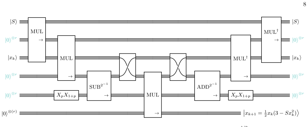
The load-bearing object is the matrix-value oracle $O_{\vartheta}$, defined by the angle formula $\vartheta_{uv}=\arccos\sqrt{|H_{uv}|/\lVert H\rVert_{\max}}$ together with the sign bit. The machinery that carries the argument is a tower of reversible fixed-point arithmetic circuits: a generic quantum adder used to build a multiplier, a Horner-scheme polynomial evaluator, a Newton–Raphson square-root routine, and Toffoli-based comparison and conjunction circuits for testing whether nodes lie inside the geometry $\Omega$ and outside the Dirichlet boundary. The identity that ties the arithmetic to the target oracle is the Taylor expansion of $\arccos\sqrt{x}$ in Eq. (4), which turns the transcendental angle into a polynomial-plus-square-root computation. The arithmetic tower determines the $r$-scaling in the final cost, while the geometry tests contribute the $N_{\mathrm{geo}}$ and $N_{\mathrm{D}}$ terms.
What would settle it
Simulate Algorithm 1 on a small one-dimensional finite element problem (e.g., $N=4$) with fixed-point registers, and compare the angle returned by the circuit with the exact value $\arccos\sqrt{|H'_{uv}|}$ for bulk, edge, and flag entries; if the difference exceeds the register's rounding error, the oracle is storing wrong angles despite the quoted complexity.
Extended reading notes
Core claim
The central claim is that the oracle $O_{\vartheta}$, which reads a matrix position $|u,v\rangle$ and outputs the sign and the angle $\vartheta_{uv}=\arccos\sqrt{|H_{uv}|/\lVert H\rVert_{\max}}$, can be built from reversible fixed-point arithmetic with polylogarithmic cost in $N$. The paper derives the stiffness and mass matrices of elastic structures from a Lagrangian, simplifies them via mass lumping and box test functions, and shows that for a homogeneous one-dimensional mesh every matrix element falls into three cases (flag, edge, bulk) whose values are constant numbers plus Kronecker-delta terms. These values feed into the Taylor expansion of $\arccos\sqrt{x}$, truncated at order $K$; the square root is computed by $L$ Newton–Raphson iterations and the polynomial by Horner's scheme. The final resource count is $O((K+L+N_{\mathrm{geo}}+N_{\mathrm{D}})r)$ ancilla qubits and $O((K+L)r^2+\log_2(N_{\mathrm{geo}}+N_{\mathrm{D}}))$ runtime, which with $r=O(\log N)$ is polylogarithmic in $N$. With that scaling, the oracle does not endanger potential polynomial or exponential quantum advantages.
Load-bearing premise
Everything rests on the Taylor expansion of $\arccos\sqrt{x}$ being accurate for every normalized matrix entry the oracle touches, yet the paper's own worked example sends entries with $x=1/4$, $1/2$, and $1$ through it, and the paper notes the expansion is poor near $x=1$ without supplying a corrected branch or an error bound.
Editorial extensions
If this is right
- For quantum algorithms that use block-encoded finite element matrices, oracle construction is asymptotically cheap: with $r=O(\log N)$ the gate count of $O_{\vartheta}$ is polylogarithmic in $N$, so the translation from query complexity to gate complexity does not erase a polynomial or exponential speedup.
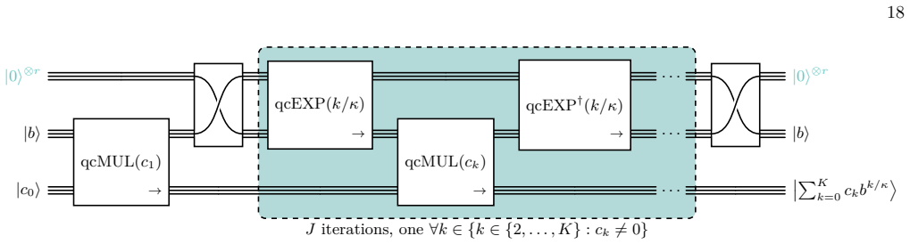
- The arithmetic subroutines—adder-based multiplication, Horner polynomial evaluation, Newton–Raphson square root, and in-place signomial exponentiation—are reusable building blocks for other quantum oracles that need elementary-function evaluations.
- The construction extends from one dimension to $d$ dimensions and to geometries approximated by hypercuboids or hyperellipsoids; only the number of geometric tests grows, through $N_{\mathrm{geo}}$ and $N_{\mathrm{D}}$, and their combined contribution is logarithmic in cost when those parameters are fixed.
- In the homogeneous one-dimensional case, Algorithm 1 gives a concrete reversible circuit from node labels $|i,j\rangle$ to $|\mathrm{sgn}_b(H_{ij}),\vartheta_{ij}\rangle$, so the oracle can be compiled and tested directly rather than left as a black box.
Reading between the lines
- If the number of geometry primitives $N_{\mathrm{geo}}$ and $N_{\mathrm{D}}$ must grow with $N$ to keep a curved or complicated boundary faithfully approximated as the mesh is refined, the $O((N_{\mathrm{geo}}+N_{\mathrm{D}})r)$ ancilla term would reintroduce $N$-dependence; the paper's polylogarithmic conclusion rests on fixing these parameters independently of $N$.
- The Taylor truncation assumption $x\ll 1$ is directly testable: the paper's own one-dimensional entries include normalized magnitudes $x=1/4$, $1/2$, and $1$, so a small simulation comparing Algorithm 1's output with the exact $\arccos\sqrt{x}$ would show whether a corrected branch is needed for practical use.
- A similar fixed-point analysis could be applied to the row-location oracle; the paper assumes regular meshes make the nonzero positions cheap via shift operations, and for unstructured meshes that part of the oracle could dominate the total cost.
Signed reviews
Editorial analysis
A structured set of objections, weighed in public.
Referee Report
Summary. The paper addresses the gate-level cost of constructing quantum matrix-element oracles for finite element method (FEM) matrices used in block-encoding. Starting from quantum adders, it develops fixed-point circuits for multiplication, polynomial evaluation via Horner's scheme, Newton-Raphson square roots, comparisons, and simple logic operations. It then applies these to a one-dimensional elastic normal-mode example, encoding the normalized matrix entry H'_ij = H_ij/||H||_max and the angle theta_uv = arccos(sqrt(|H_uv|/||H||_max)). The central claim is that, with r = O(log N) and K, L, N_geo, N_D treated as independent of N, the oracle O_theta uses O((K+L+N_geo+N_D)r) ancilla qubits and runs in time O((K+L)r^2 + log(N_geo+N_D)), so oracle construction does not destroy potential polynomial or exponential quantum advantages in N.
Significance. If correct, the paper fills a real gap: many quantum algorithms for FEM or PDEs are analyzed only in the query model, and explicit reversible-arithmetic constructions with ancilla and runtime counts are valuable. The modular adder-based presentation and the detailed accounting for polynomial, square-root, and geometry subroutines are genuine strengths, and the resource counting for the arithmetic blocks is internally consistent and grounded in the cited adder literature. However, the correctness of the central object O_theta rests on the evaluation of arccos(sqrt(x)), and the only implemented evaluation is the truncated Taylor series in Eq. (4). That series is misprinted, and it is used for normalized matrix entries as large as x = 1/2 and x = 1 in the paper's own motivating example, despite the stated small-x assumption. The polylogarithmic oracle-cost claim is therefore not yet supported for the example the paper itself presents.
major comments (3)
- [§I, Eq. (4)] The Taylor expansion in Eq. (4) has incorrect coefficients. The correct expansion is arccos(sqrt(x)) = pi/2 - x^(1/2) - (1/6)x^(3/2) - (3/40)x^(5/2) - (5/112)x^(7/2) - ..., while the printed terms with prefactors 3/40 and 5/112 are shifted by one power. Since the polynomial routine POLY in Section II B is applied with these coefficients, the implemented circuit evaluates a function that is not arccos(sqrt(|H'|)), even in the regime where the truncation is otherwise valid.
- [§IV B, Algorithm 1 and Eq. (60)] The small-x justification for the truncated expansion fails on the paper's own example. Equation (60) and Algorithm 1 produce normalized entries |H'_ij| equal to 1/4, 1/2, and 1 (the latter for the flag rows), while Section I restricts the expansion to x << 1 and explicitly concedes it is not accurate for x near 1. For x = 1 the exact value is arccos(1) = 0, whereas the truncated series in Eq. (4) gives a value near pi/2 - 1, i.e. about 0.57. Algorithm 1 contains no branch for large x, and the replacement formula mentioned in Section I is not implemented or costed, so the circuit as printed is not a faithful oracle for the motivating matrix.
- [§IV B, Eqs. (74)–(77)] No error bound is supplied that connects the truncation order K, the Newton-Raphson iteration count L, the fixed-point precision r, and the final error in theta. This is load-bearing because the downstream block-encoding and quantum phase estimation require theta to be encoded to a controlled accuracy; without such a bound, the resource statements in Eqs. (76) and (77) are not a correctness-preserving complexity statement for O_theta.
minor comments (4)
- [§I, Eq. (4)] The notation sqrt(x)^3 and sqrt(x)^5 is ambiguous; since the expansion is in powers of sqrt(x), the terms should be written x^(3/2) and x^(5/2) (and, after the coefficient correction, x^(7/2) as well).
- [§I] The proposed alternative identity appears to be a typo: arccos(sqrt(x)) equals 2 arcsin(sqrt((1 - sqrt(x))/2)), not the printed expression involving (1-x)/2; the printed expression is not equal to arccos(sqrt(x)) at x = 0.
- [§IV B, Eqs. (67)–(68)] The serial and parallelized versions of the geometry-condition runtime are both discussed, but the final runtime in Eq. (77) uses the parallelized form without restating the assumption; it would be clearer to explicitly carry the serial form t_geo = O((N_geo + N_D) r) into the comparison with Eq. (77).
- [Algorithm 1] The flag assignment H' <- |delta_ij| silently uses the choice ||H||_max = F; the text states this only implicitly through Eq. (61), so a reader could miss that the flag rows are normalized to exactly 1.
Circularity Check
No significant circularity: the oracle cost is a bottom-up composition of external arithmetic primitives, with only a non-load-bearing self-citation.
full rationale
The paper's central derivation is a bottom-up composition of externally established arithmetic primitives: quantum adders (Refs. [23-27,31]), multipliers built from adders, Horner-scheme polynomials, and Newton-Raphson square root. The oracle complexity O((K+L)r^2 + log(Ngeo+ND)) is obtained by summing the published runtimes of these routines, and it does not reuse the conclusion it targets. The only self-citation, Ref. [18], supplies the application context (response functions of coupled oscillators) and the requirement that the oracle be polylogarithmic; it is not used to justify any circuit construction or complexity bound. Equation (4) is a Taylor expansion of arccos(sqrt(x)) with fixed coefficients, and Algorithm 1's H' values are derived independently from the FEM mass and stiffness matrices, so the oracle's cost is not a fitted parameter renamed as a prediction. The acknowledged inaccuracy of the truncated expansion for x near 1, including the paper's own x=1/2 and x=1 entries, is a correctness limitation of the printed circuit, not a circularity: the stated complexity still describes the circuit as specified, and the expansion is not defined in terms of the oracle's output. Therefore no step in the derivation chain reduces to its own input or to a load-bearing self-citation.
Assumptions & free parameters
free parameters (4)
- K =
truncation order, input to construction
- L =
Newton-Raphson iteration count, input to construction
- r =
O(log N)
- p =
binary point position, chosen in [0,r]
assumptions (4)
- ad hoc to paper The truncated Taylor expansion in Eq. (4) accurately approximates arccos(sqrt x) for the normalized entries produced by Algorithm 1.
- domain assumption Fixed-point arithmetic with r qubits and binary point p computes H', sqrt, and theta with negligible error for the QPE application.
- domain assumption The Newton-Raphson square root converges for every value of |H'| generated by the comparisons.
- domain assumption FEM stiffness and mass matrices for elastic normal mode analysis are well represented by the mass-lumped, hypercuboid-approximated form in Eqs. (52) and (58).
Cite this review
Pith. "Pith review of Quantum oracles for the finite element method." pith.science (2026). https://pith.science/paper/LQVUWDPM
@misc{pith2026250419827,
  author       = {Pith},
  title        = {Pith review of: Quantum oracles for the finite element method},
  year         = {2026},
  howpublished = {\url{https://pith.science/paper/LQVUWDPM}},
  note         = {Machine review of arXiv:2504.19827}
}
abstract
In order to assess potential advantages of quantum algorithms that require quantum oracles as subroutines, the careful evaluation of the overall complexity of the oracles themselves is crucial. This study examines the quantum routines required for the implementation of oracles used in the block-encoding of the $N \times N$ stiffness and mass matrices, which typically emerge in the finite element analysis of elastic structures. Starting from basic quantum adders, we show how to construct the necessary oracles, which require the calculation of polynomials, square root and the implementation of conditional operations. We propose quantum subroutines based on fixed-point arithmetic that, given an $r$-qubit register, construct the oracle using $\mathcal{O}((K + L + N_{\mathrm{geo}} + N_{\mathrm{D}}) r)$ ancilla qubits and have a $\mathcal{O}((K + L)r^2 + \log_2(N_{\mathrm{geo}} + N_{\mathrm{D}}))$ runtime, with $K$ the order at which we truncate the polynomials, $L$ the number of iterations in the Newton-Raphson subroutine for the square root, while $N_{\mathrm{geo}}$ and $N_{\mathrm{D}}$ are the number of hypercuboids used to approximate the geometry and the boundary, respectively. Since in practice $r$ scales as $r = \mathcal{O}(\log_2 N)$, and assuming that the other parameters are fixed independently of $N$, this shows that the oracles, while still costly in practice, do not endanger potential polynomial or exponential advantages in $N$.
Figures


Figures from the paper (11 more)





Reference graph
Works this paper leans on
- [19]
- [20]
-
[18]
S. Danz, M. Berta, S. Schröder, P. Kienast, F. K. Wilhelm, and A. Ciani, Calculating response functions of coupled oscillators using quantum phase estimation, arXiv e-prints , arXiv:2405.08694 (2024)
arXiv 2024
-
[1]
D. Deutsch and R. Penrose, Quantum theory, the Church–Turing principle and the universal quantum com- puter, Proceedings of the Royal Society of London. A. Mathematical and Physical Sciences400, 97 (1985)
work page 1985
-
[2]
Deutsch and R
D. Deutsch and R. Jozsa, Rapid solution of problems by quantum computation, Proceedings of the Royal Society of London. Series A: Mathematical and Physical Sciences 439, 553 (1992)
1992
-
[3]
L. K. Grover, A fast quantum mechanical algorithm for database search, inProceedings of the Twenty-Eighth An- nual ACM Symposium on Theory of Computing , STOC ’96 (Association for Computing Machinery, New York, NY, USA, 1996) p. 212–219
work page 1996
-
[4]
J. M. Martyn, Z. M. Rossi, A. K. Tan, and I. L. Chuang, Grand Unification of Quantum Algorithms, PRX Quan- tum 2, 040203 (2021)
work page 2021
-
[5]
A. Gilyén, Y. Su, G. H. Low, and N. Wiebe, Quantum Singular Value Transformation and beyond: Exponential Improvements for Quantum Matrix Arithmetics, inPro- ceedings of the 51st Annual ACM SIGACT Symposium on Theory of Computing , STOC 2019 (Association for Computing Machinery, New York, NY, USA, 2019) p. 193–204
work page 2019
Show all 56 references
-
[6]
A. M. Dalzell, S. McArdle, M. Berta, P. Bienias, C.- F. Chen, A. Gilyén, C. T. Hann, M. J. Kastoryano, E. T. Khabiboulline, A. Kubica, G. Salton, S. Wang, and F. G. S. L. Brandão, Quantum algorithms: A sur- vey of applications and end-to-end complexities, arXiv e-prints , arXi...
2023 arXiv
-
[7]
G. H. Low and I. L. Chuang, Optimal Hamiltonian Sim- ulation by Quantum Signal Processing, Phys. Rev. Lett. 118, 010501 (2017)
2017
-
[8]
G. H. Low and I. L. Chuang, Hamiltonian Simulation by Qubitization, Quantum3, 163 (2019)
2019
-
[9]
A. M. Childs, On the Relationship Between Continuous- and Discrete-Time Quantum Walk, Commun. Math. Phys 294, 581 (2010)
2010
-
[10]
D. W. Berry and A. M. Childs, Black-Box Hamiltonian Simulation and Unitary Implementation, Quantum Infor- mation and Computation12, 29–62 (2012)
2012
-
[11]
Fish and T
J. Fish and T. Belytschko, A First Course in Finite Elements (Wiley, 2007)
2007
-
[12]
Ern and J.-L
A. Ern and J.-L. Guermond, Theory and Practice of Finite Elements, Applied Mathematical Sciences, Vol. 159 (Springer, New York, 2004)
2004
-
[13]
Bathe, Finite Element Procedures (Prentice Hall, 2006)
K. Bathe, Finite Element Procedures (Prentice Hall, 2006)
2006
-
[14]
R. Cook, D. Malkus, and M. Plesha,Concepts and Appli- cations of Finite Element Analysis (Wiley, 1989)
1989
-
[15]
S. S. Rao, The Finite Element Method in Engineering (Butterworth-Heinemann, 2005)
2005
-
[16]
B. D. Clader, B. C. Jacobs, and C. R. Sprouse, Precon- ditioned Quantum Linear System Algorithm, Phys. Rev. Lett. 110, 250504 (2013)
2013
-
[17]
Montanaro and S
A. Montanaro and S. Pallister, Quantum algorithms and the finite element method, Phys. Rev. A 93, 032324 (2016)
2016
-
[21]
Vedral, A
V. Vedral, A. Barenco, and A. Ekert, Quantum networks for elementary arithmetic operations, Phys. Rev. A54, 147 (1996)
1996
-
[22]
Beckman, A
D. Beckman, A. N. Chari, S. Devabhaktuni, and J. Preskill, Efficient networks for quantum factoring, Phys. Rev. A54, 1034 (1996)
1996
-
[23]
S. A. Cuccaro, T. G. Draper, S. A. Kutin, and D. Petrie Moulton, A new quantum ripple-carry addition circuit, arXiv e-prints , quant-ph/0410184 (2004)
2004 arXiv
-
[24]
M. K. Thomsen and H. B. Axelsen, Parallel optimization of a reversible (quantum) ripple-carry adder, inUncon- ventional Computing, edited by C. S. Calude, J. F. Costa, R. Freund, M. Oswald, and G. Rozenberg (Springer Berlin Heidelberg, Berlin, Heidelberg, 2008) pp. 228–241
2008
-
[25]
Van Meter and K
R. Van Meter and K. M. Itoh, Fast quantum modular exponentiation, Phys. Rev. A71, 052320 (2005). 15
2005
-
[26]
T. G. Draper, S. A. Kutin, E. M. Rains, and K. M. Svore, A logarithmic-depth quantum carry-lookahead adder, arXiv e-prints , quant-ph/0406142 (2004)
2004 arXiv
-
[27]
Ruiz-Perez and J
L. Ruiz-Perez and J. C. Garcia-Escartin, Quantum arith- metic with the quantum Fourier transform, Quantum Information Processing16, 152 (2017)
2017
-
[28]
Gidney, Halving the cost of quantum addition, Quan- tum 2, 74 (2018)
C. Gidney, Halving the cost of quantum addition, Quan- tum 2, 74 (2018)
2018
-
[29]
Zalka, Fast versions of Shor’s quantum factoring algo- rithm, arXiv e-prints , quant-ph/9806084 (1998)
C. Zalka, Fast versions of Shor’s quantum factoring algo- rithm, arXiv e-prints , quant-ph/9806084 (1998)
1998 arXiv
-
[30]
T. G. Draper, Addition on a Quantum Computer, arXiv e-prints , quant-ph/0008033 (2000)
2000 arXiv
-
[31]
Paler, Quantum Fourier addition simplified to Toffoli addition, Phys
A. Paler, Quantum Fourier addition simplified to Toffoli addition, Phys. Rev. A106, 042444 (2022)
2022
-
[32]
F. Orts, G. Ortega, and E. M. Garzón, An optimized quantum circuit for converting from sign–magnitude to two’s complement, Quantum Information Processing18, 332 (2019)
2019
-
[33]
Rieffel and W
E. Rieffel and W. Polak,Quantum Computing: A Gen- tle Introduction, Scientific and Engineering Computation (MIT Press, 2014)
2014
-
[34]
Thapliyal, T
H. Thapliyal, T. S. S. Varun, E. Munoz-Coreas, K. A. Britt, and T. S. Humble, Quantum Circuit Designs of Integer Division Optimizing T-Count and T-Depth, in 2017 IEEE International Symposium on Nanoelectronic and Information Systems (iNIS) (2017) pp. 123–128
2017
-
[35]
S. S. Gayathri, R. Kumar, S. Dhanalakshmi, G. Dooly, and D. B. Duraibabu, T-Count Optimized Quantum Cir- cuit Designs for Single-Precision Floating-Point Division, Electronics 10 (2021)
2021
-
[36]
S. S. Gayathri, R. Kumar, and S. Dhanalakshmi, Efficient Floating-point Division Quantum Circuit using Newton- Raphson Division, Journal of Physics: Conference Series 2335, 012058 (2022)
2022
-
[37]
Flynn, On Division by Functional Iteration, Comput- ers, IEEE Transactions onC-19, 702 (1970)
M. Flynn, On Division by Functional Iteration, Comput- ers, IEEE Transactions onC-19, 702 (1970)
1970
-
[38]
Bampi and A
F. Bampi and A. Morro, A lagrangian density for the dynamics of elastic dielectrics, International Journal of Non-Linear Mechanics18, 441 (1983)
1983
-
[39]
G. A. Holzapfel, Nonlinear Solid Mechanics: A Continuum Approach for Engineering Science, Meccanica37, 489 (2002)
2002
-
[40]
J. F. Nye,Physical Properties of Crystals - Their Rep- resentation by Tensors and Matrices (Clarendon Press, Oxford, 1985)
1985
-
[41]
M. T. Dove, Acoustic modes and macroscopic elasticity, in Introduction to Lattice Dynamics , Cambridge Topics in Mineral Physics and Chemistry (Cambridge University Press, 1993) p. 95–100
1993
-
[42]
D. Han, H. H. Dai, and L. Qi, Conditions for Strong Ellipticity of Anisotropic Elastic Materials, Journal of Elasticity 97, 1 (2009)
2009
-
[43]
Huang and L
Z.-H. Huang and L. Qi, Positive definiteness of paired symmetric tensors and elasticity tensors, Journal of Com- putational and Applied Mathematics338, 22 (2018)
2018
-
[44]
M. H. Sadd,Elasticity: Theory, applications, and numer- ics (Academic Press, 2014)
2014
-
[45]
A. F. Bower, Applied Mechanics of Solids (CRC Press LLC, 2010)
2010
-
[46]
Felippa, Introduction to Finite Element Methods (Uni- versity of Colorado, Boulder, 2004)
C. Felippa, Introduction to Finite Element Methods (Uni- versity of Colorado, Boulder, 2004)
2004
-
[47]
P. W. Shor, Polynomial-Time Algorithms for Prime Fac- torization and Discrete Logarithms on a Quantum Com- puter, SIAM Journal on Computing26, 1484 (1997)
1997
-
[48]
Beauregard, Circuit for Shor’s algorithm using 2n+3 qubits, Quantum Info
S. Beauregard, Circuit for Shor’s algorithm using 2n+3 qubits, Quantum Info. Comput.3, 175–185 (2003)
2003
-
[49]
Pavlidis and D
A. Pavlidis and D. Gizopoulos, Fast quantum modular exponentiation architecture for Shor’s factoring algorithm, Quantum Info. Comput.14, 649–682 (2014)
2014
-
[50]
Parker and J
A. Parker and J. Hamblen, Optimal value for the Newton- Raphson division algorithm, Information Processing Let- ters 42, 141 (1992)
1992
-
[51]
Barenco, C
A. Barenco, C. H. Bennett, R. Cleve, D. P. DiVincenzo, N. Margolus, P. Shor, T. Sleator, J. A. Smolin, and H. Weinfurter, Elementary gates for quantum compu- tation, Phys. Rev. A52, 3457 (1995). Appendix A: Fixed-point exponentiation In this appendix, we describe how to contin...
1995
-
[52]
Computation off(a) with the out-of-place arith- metic operatorUf Uf|a, 0⟩ =|a,f (a)⟩. (B1)
-
[53]
Swap of the target and input register SWAP|a,f (a)⟩ =|f(a),a⟩. (B2)
-
[54]
(B3) In this section, we describe the two in-place operations inSQ and inMUL, occurring in the exponentiator in Sec- tion IIB
Annihilation of the input a with the Hermitian conjugate U† f−1: U† f−1|f(a),a⟩ =|f(a), 0⟩. (B3) In this section, we describe the two in-place operations inSQ and inMUL, occurring in the exponentiator in Sec- tion IIB. 18 J iterations, one∀k∈{k∈{ 2,...,K } :ck̸= 0} ... ... ......
-
[55]
For two registers of r qubits each (focusing on positive numbers,a,b> 0), we apply a series ofr CNOT gates between qubit pairs of equal significance (see Fig
Comparisons In order to compare two binary numbers (a and b) stored in the computational basis of two quantum regis- ters, we can make use of CNOT gates. For two registers of r qubits each (focusing on positive numbers,a,b> 0), we apply a series ofr CNOT gates between qubit pa...
-
[56]
(60) requires the combination of multiple compar- isons
Boolean logical operations Eq. (60) requires the combination of multiple compar- isons. This can be achieved with the conjunction (∧, and). The Toffoli gate is the natural quantum implementation of the conjunction as it inverts the information in the target qubit only if both ...
Reviewed August 16, 2026 · model on record in the stance chip above.
Discussion (0). Continue with ORCID to comment.