LSTM-based Flow Prediction

Hongzhi Wang; Shihan Tang; Yang Song

REVIEW 6 major objections 5 minor 13 references

LSTM-based Flow Prediction

T0 review · 6 major / 5 minor · reviewed 2026-08-14 · deepseek-v4-flash

Challenge this review Re-run · record.json Download PDF Read on arXiv ↗ Review JSON

Pith's one-line read This paper claims that adding multivariate tuning to LSTM cuts flow-prediction RMSE by 54.05% on an industrial boiler dataset.

desk verdict The method is a reasonable engineering combination, but the 54.05% improvement claim is unsupported by an unfair baseline and test-set selection. read the letter →

arxiv 1908.03571 v1 pith:LTQM2LTB submitted 2019-08-09 cs.LG eess.SPstat.ML

Hongzhi Wang , Yang Song , Shihan Tang This is my paper · ORCID

classification cs.LGeess.SPstat.ML

keywords LSTMtimeseriespredictionflowindustrialdatamultivariatetuningperiodicanalysisrootmeansquareerrorrandomforestfeatureselection

verification ladder T0 review T1 audit T2 compute T3 formal

The pith

A machine-rendered reading of the paper's core claim, the machinery that carries it, and where it could break.

The reading

This paper tries to establish that flow prediction on industrial time-series data improves substantially when a long short-term memory network is combined with a multivariate tuning pipeline. On a real boiler dataset with 70 sensor dimensions, the proposed method reports a root-mean-square error of 9.13, compared with 19.87 for a plain LSTM, a 54.05% reduction, and it also beats random forest, backpropagation, and CNN baselines. The authors argue that industrial data's hidden periodicity and cross-variable dependencies are the reasons LSTM alone underperforms, and that their tuning modules address exactly those two features. If the claim holds, factories could forecast output or flow more reliably and detect equipment problems earlier with a modest algorithmic change.

What carries the argument

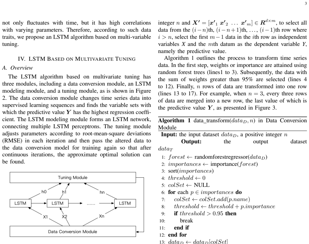
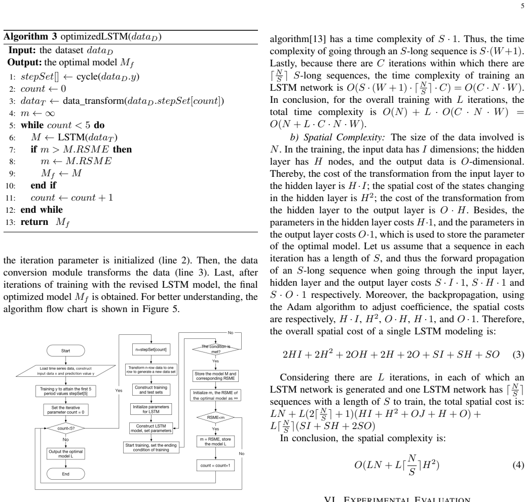
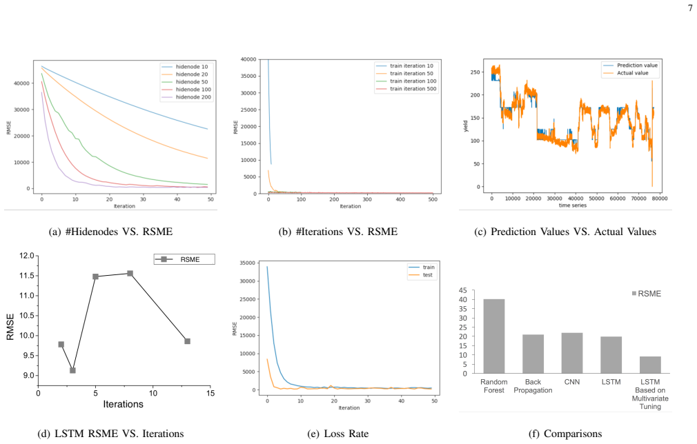
The load-bearing object is the tuning module's period detection: the target series is normalized to the (0,1) interval, the positions where the sign of the value flips are recorded, the distances between flips define candidate period lengths, and the five smallest such lengths are used as window sizes n in the data reshaping step. This turns an opaque, hard-to-guess hyperparameter—how many past rows to feed the LSTM—into a quantity read off the data itself. The same module then trains an LSTM for each candidate period and selects the model with the minimum RMSE, which the paper treats as an approximate optimum with reduced overfitting risk.

What would settle it

Retrain the original LSTM using the same hyperparameters the proposed method was tuned to—sequence length 500, 100 hidden nodes, and 50 iterations—on the same train/test split; if its RMSE falls to roughly 9-10, the 54.05% improvement is primarily hyperparameter tuning and not the multivariate or periodic modules.

Watch

Extended reading notes

Core claim

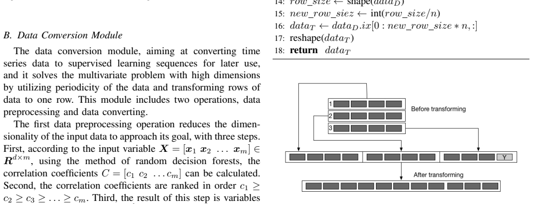
The central discovery is an algorithmic recipe: convert multivariate time series into supervised sequences by selecting the top variables via random-forest importance (covering 95% of cumulative importance) and reshaping n consecutive rows into one training row; train a single-layer LSTM on those sequences; then, instead of guessing a window size, detect the signal's period by recording zero-crossings of the normalized target variable, take the five shortest period values, and iterate training over those window sizes, keeping the model with the lowest RMSE. On the industrial boiler dataset this pipeline reaches RMSE 9.13, and the paper attributes the gain to the periodic window selection plus the multivariate transformation. The authors also argue the chosen model is not overfitting because the training and test loss curves converge.

Load-bearing premise

The comparison rests on the assumption that the 'original LSTM' baseline was run with a fair, comparable hyperparameter configuration, but the paper never reports that baseline's window size, hidden nodes, or iteration count.

Editorial extensions

If this is right

If the reported RMSE reduction holds under matched baselines, adopting the tuning pipeline should improve flow forecasting in settings where LSTM is already deployed, without changing the core network architecture.
The zero-crossing period detector gives a data-driven rule for choosing the look-back window, replacing manual selection and plausibly transferring to other periodic industrial signals such as pressure or temperature.
The random-forest feature selection step shrinks 70 sensor dimensions to a 95%-importance subset, so the method should also reduce training cost and model complexity relative to training on all dimensions.
Selecting the best of five candidate window sizes by validation RMSE provides a built-in guard against picking a poor window, though the 'first five smallest periods' rule is an arbitrary cap.

Reading between the lines

Editorial extensions of the paper, not claims the author makes directly.

A matched-hyperparameter comparison would likely shrink the gap: plain LSTM is known to be sensitive to look-back length and hidden size, so the head-to-head claim needs the baseline tuned to the same budget to be credible.
The period-detection rule assumes the normalized target alternates sign; for strictly positive flows that never cross zero, the algorithm would record no flips, so a practical extension would need a detrending or baseline-subtraction step.
The same modular recipe—feature selection, window-from-periodicity, iterative RMSE selection—could be lifted onto other sequence models such as GRU or temporal convolutional networks; the paper does not test this, but nothing in the modules is LSTM-specific beyond the network itself.
The paper's 'no overfitting' argument relies on loss-curve convergence and on averaging over five periods; a stronger test would be a true held-out time block from a later date, since the random split leaks neighboring timestamps across train and test.

Share X Bluesky LinkedIn Reddit HN

Signed reviews

No signed human review yet.

Editorial analysis

A structured set of objections, weighed in public.

Desk editor's note, referee report, and a circularity audit.

Desk Editor's Note

read the letter

Punchline: this is a reject for me, but not because the idea is crazy. The proposed LSTM pipeline — random-forest feature selection, zero-crossing period detection, and candidate window sizes — is a sensible engineering approach for multivariate industrial time series. The trouble is the evaluation: the headline 54.05% improvement is built on an unspecified baseline, test-set selection, and no error bars.

What's actually new: the specific combination is not in the cited literature, and it's a reasonable integration of standard pieces. The complexity analysis is explicit, and the authors identify real challenges — opaque periodicity and multivariate dependence. If I were an engineer with this boiler dataset, I might try their pipeline. There is value in that.

But the soft spots are load-bearing. The "original LSTM" baseline in Table VII is never given hyperparameters, while the proposed method's settings were tuned on test RMSE in Tables III–V. An untuned LSTM could easily give 19.87; a tuned LSTM might come close to 9.13. So the claimed 54.05% improvement is unsupported. Algorithm 3 also fits five LSTM models for the five smallest detected periods and returns the one with lowest RMSE; if that RMSE is computed on the test partition, it is selection on the test set. The paper's statement that training/test loss curves "prove" no overfitting does not address this. There are internal contradictions too: Table IV shows 200 hidden nodes gives RMSE 8.69, yet the text says 100 is better; Table III shows sequence length changing RMSE from 22.83 to 11.49, yet the text says it has small influence. That suggests the narrative was written after the results.

Who this is for: practitioners wanting a quick, interpretable way to add periodicity and feature selection to LSTM. As a paper, it needs a matched baseline, repeated runs with error bars, and evaluation on more than one dataset. I wouldn't desk-reject the topic, but I also wouldn't accept this version.

Recommendation: send it to peer review only if you expect a referee to demand a redone experiment section. The underlying idea is fine, but the central claim is currently unsubstantiated.

Referee Report

6 major / 5 minor

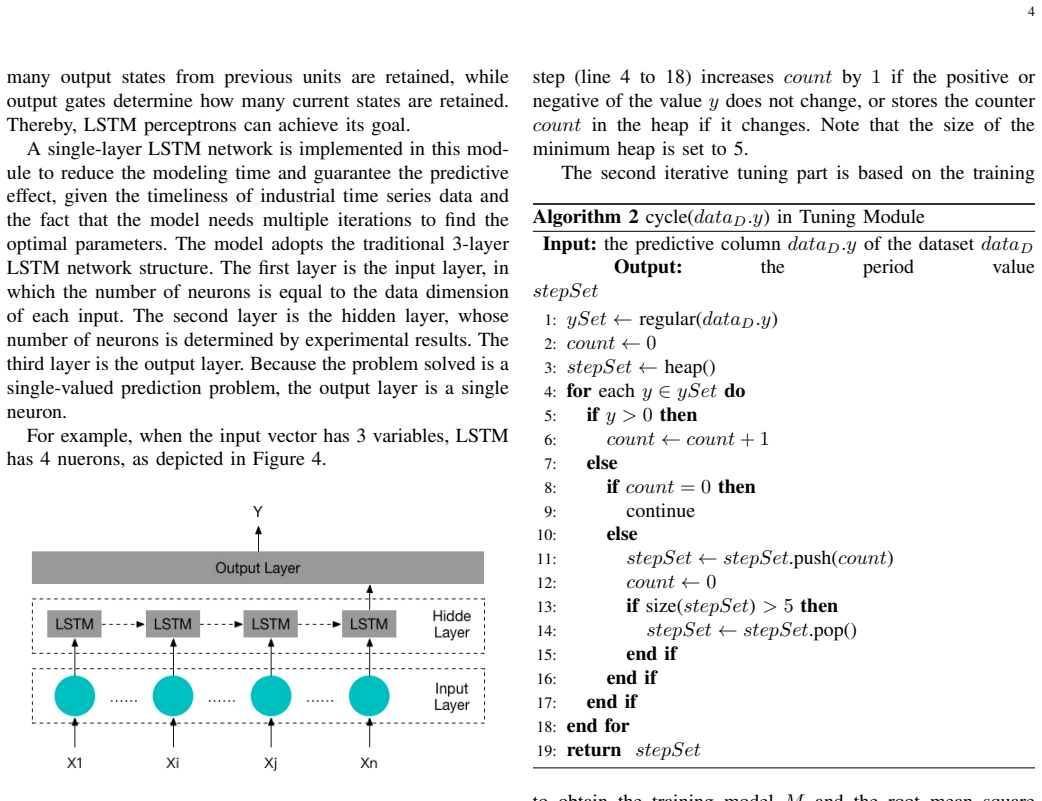
Summary. The paper proposes an LSTM-based prediction method for industrial flow data, termed 'LSTM based on multivariate tuning.' The method consists of three modules: a data conversion module that uses random forest importance to reduce dimensionality and converts time series into supervised sequences with a window size n; an LSTM modeling module; and a tuning module that estimates candidate periods from zero-crossings of a normalized target and iterates over the five smallest detected periods, selecting the model with the smallest RMSE. The central claim is that on a 70-dimensional industrial boiler dataset with over 400,000 records, the proposed method achieves an RMSE of 9.13 versus 19.87 for a 'traditional LSTM,' a claimed 54.05% improvement. The paper also provides time and space complexity analyses and describes the experimental tuning of sequence length, hidden-layer nodes, and number of iterations.

Significance. Should the empirical claim hold, the proposed method would be a practically relevant contribution to industrial time-series prediction, as it addresses periodicity and multivariate dependency, and the complexity analysis is a useful addition. The paper also gives concrete algorithms and a real-world evaluation. However, the evaluation as presented does not support the central claim: the baseline comparison is not matched, the reported 'optimal' parameters are contradicted by the paper's own tuning table, the model-selection procedure is biased, and no error bars or repeated runs are provided. The internal inconsistencies in the period-detection and pseudocode would need to be resolved before the method is reproducible. The contribution is therefore not yet established at the level expected for a journal publication.

major comments (6)

[VI.D / Table VII] The comparison between the proposed method and 'original LSTM' in Table VII is not a controlled experiment. The hyperparameters of the LSTM baseline are never specified, whereas the proposed method's sequence length, hidden-layer size, and iteration count were explicitly tuned in Section VI.C. Table III shows that setting the sequence length to 500 with hidden size 50 already yields an RMSE of 11.49, nearly halving the reported baseline of 19.87, so the claimed 54.05% improvement could be an artifact of hyperparameter selection rather than of the multivariate-tuning modules. The authors should compare against an LSTM with the same tuned hyperparameters (e.g., 500/100/50) and report error bars over multiple random seeds.
[VI.C / Table IV] Table IV reports that Experiment 10 (sequence length 500, 200 hidden-layer nodes, 50 iterations) achieves RMSE 8.69, which is lower than the RMSE of 9.13 for Experiment 9 with 100 hidden-layer nodes. Nevertheless, the text states that 100 hidden nodes 'can achieve a better experimental result' and later designates 500/100/50 as the optimal parameters. This contradicts the paper's stated objective of minimizing RMSE and renders the tuning process and the headline 9.13 result internally inconsistent; the authors need to explain why the lower-RMSE configuration was not used.
[IV.D / Algorithm 3] Algorithm 3 selects the model with minimal RMSE among the five smallest detected periods. If the RMSE used in this comparison is computed on the test partition, then the reported 9.13 is the result of fitting to the test set via model selection, and the claim in Section IV.D that 'there is no overfitting' from considering only five periods does not address this selection bias. The loss-curve argument in Section VI.C is also not a statistical test of overfitting and does not justify using the selected minimum without a correction (e.g., nested validation or a model-selection test).
[IV.D / Algorithm 2] The period-detection procedure is internally inconsistent: the text says the predictive values are normalized into the (0,1) interval, but Algorithm 2 then detects periods by counting steps until the sign of y changes (y > 0 versus else). If all values lie in (0,1), every y is positive, count never resets, and stepSet remains empty, so Algorithm 3 would fail at line 3. The normalization must be redefined (e.g., zero-mean standardization) or the detection logic must be changed; as written, the proposed algorithm is not implementable.
[V.A / Algorithm 3] In Algorithm 3, the variable dataT is computed once before the loop (line 3) using stepSet[count] with count=0, and is never recomputed inside the while loop. Consequently, the loop trains an LSTM on the same transformed data for all five iterations instead of using each of the five period candidates, contradicting the textual description in Section IV.D and Section VI.C. This is a load-bearing discrepancy in the algorithm's presentation and must be corrected.
[VI.B-C] All reported RMSE values in Tables III–VII are single numbers with no standard deviations, confidence intervals, or number of repeated runs, despite the statement in Section VI.B that 'the experiment reduces the experimental error by multiple measurements and averaging.' Because LSTM training is stochastic, the claimed 54.05% improvement cannot be assessed without such information. At minimum, the authors should provide the mean and standard deviation over several independent runs for each configuration.

minor comments (5)

[Throughout] The acronym RMSE is consistently misspelled 'RSME' throughout the manuscript, including equations and tables.
[IV.B / Algorithm 1] Algorithm 1 line 15 contains the typo 'new row siez' and the reshape operation is not specified precisely.
[IV.D] Section IV.D says the first five periods are 'taken as the number of iterations'; they are actually candidate window sizes n, not iteration counts.
[VI.C] Several sentences are ungrammatical, e.g., 'the number of iterations will be It is tentatively set to 50 times' in Section VI.C; a thorough language edit is needed.
[VI.C] Figure and table numbering is inconsistent; for example, Section VI.C refers to 'Figure 6' while the optimal-prediction plot is labeled 'Figure 8'.

Circularity Check

0 steps flagged · score 0.0 of 10

No significant circularity: the reported RMSE values are empirical measurements and model-selection outcomes, not quantities defined in terms of the claims they support.

full rationale

The paper's central claims are experimental rather than derived. Section IV.C defines an LSTM network, Section IV.D defines periodic analysis and iterative tuning, and Algorithm 3 trains several LSTM models for the five smallest detected periods and keeps the model with minimum RMSE ('if m > M.RSME then m <- M.RSME'). The reported RMSE of 9.13 is the measured error of the selected model, not a quantity obtained by substituting the claimed conclusion into its premise. The comparison with the 'original LSTM' (RMSE 19.87 in Table VII) is likewise an empirical comparison between experiment runs; the paper never defines the proposed RMSE in terms of the baseline RMSE or vice versa. No load-bearing self-citation appears: the only external algorithm cited, Adam [13], is a standard optimizer and is not used to justify the paper's central claim. There is no imported uniqueness theorem and no ansatz smuggled in through a citation. The main legitimate concerns are statistical and methodological: the hyperparameters of the baseline 'original LSTM' are never specified, and the proposed method's hyperparameters and window length are selected using the same RMSE metric that is later reported. These issues bear on the fairness and generalizability of the 54.05% improvement claim, but they do not make the derivation circular because the reported numbers are measurements, not constructions that presuppose the conclusion.

Assumptions & free parameters 4 free parameters · 4 assumptions · 0 invented entities

The central claim rests on four tuned hyperparameters (window size, hidden nodes, iterations, feature threshold) and on three assumptions: the reliability of random forest feature importance, the zero-crossing periodicity heuristic, and the representativeness of the single dataset. No new physical or mathematical entities are introduced.

free parameters (4)

window size n = 3 (selected as best among candidate periods)
The tuning module computes the five smallest zero-crossing periods of the target and iterates LSTM over these values, keeping the model with minimum RMSE (Algorithm 3). n=3 gave the best RMSE.
number of hidden layer nodes = 100
Tuned in Section VI.C, Table IV; values 10, 20, 50, 100, 200 were tested and 100 chosen as a compromise between RMSE and training time.
number of training iterations = 50
Tuned in Section VI.C, Table V; values 10, 50, 100, 500 tested; 50 chosen because larger values did not improve RMSE.
feature selection threshold = 95% cumulative random forest importance
Section IV.B sets the threshold at 95% without justification; it controls how many sensor variables are kept.

assumptions (4)

standard math LSTM training with Adam optimization and backpropagation as described in prior work
The paper relies on the standard LSTM formulation (equations in Section II) and Adam (reference [13]) without re-deriving them.
domain assumption Random forest feature importance reflects predictive relevance of variables
Section IV.B uses random forest importances to select variables; this assumes the importance ranking is stable and meaningful for the LSTM model.
ad hoc to paper Zero crossings of the normalized target reliably estimate the period of industrial flow data
Section IV.D uses zero crossings to define periods. This is a heuristic introduced in this paper with no validation against synthetic or known-period data.
domain assumption The industrial boiler dataset is representative and correctly measured
Section VI.B describes the dataset, but no details of sensor calibration, missing data handling, or train/test split seeding are given.

how reviews work

0 comments

Cite this review

Pith. "Pith review of LSTM-based Flow Prediction." pith.science (2026). https://pith.science/paper/LTQM2LTB

@misc{pith2026190803571,
  author       = {Pith},
  title        = {Pith review of: LSTM-based Flow Prediction},
  year         = {2026},
  howpublished = {\url{https://pith.science/paper/LTQM2LTB}},
  note         = {Machine review of arXiv:1908.03571}
}

read the original abstract

In this paper, a method of prediction on continuous time series variables from the production or flow -- an LSTM algorithm based on multivariate tuning -- is proposed. The algorithm improves the traditional LSTM algorithm and converts the time series data into supervised learning sequences regarding industrial data's features. The main innovation of this paper consists in introducing the concepts of periodic measurement and time window in the industrial prediction problem, especially considering industrial data with time series characteristics. Experiments using real-world datasets show that the prediction accuracy is improved, 54.05% higher than that of traditional LSTM algorithm.

Figures

Figures reproduced from arXiv: 1908.03571 by the authors.

**Figure 1.** LSTM Neuron the unit, which is designed with a structure called a gate to modify the state by adding or removing certain information. Besides, the gate can filter the input and contains layers such as sigmoid pointwise. Sigmoid controls the amount of the input data allowed to pass, whose value is between 0 and 1. Obviously, 0 blocks all information, while 1 allows any amount to pass. The LSTM uses a three-door struc… view at source ↗

**Figure 2.** LSTM based on multivariate tuning B. Data Conversion Module The data conversion module, aiming at converting time series data to supervised learning sequences for later use, and it solves the multivariate problem with high dimensions by utilizing periodicity of the data and transforming rows of data to one row. This module includes two operations, data preprocessing and data converting. The first data preprocessing … view at source ↗

**Figure 3.** Data Transforming C. LSTM Modeling Module The LSTM modeling module connects multiple LSTM perceptrons to form an LSTM network, aiming to preserve the impact of early emerging information and connect it to the present task. LSTM perceptrons control output states, using forget gates and input gates, where forget gates determine how [PITH_FULL_IMAGE:figures/full_fig_p003_3.png] view at source ↗

Figures from the paper (4 more)

**Figure 4.** Figure 4: Single-Layer LSTM Network Structure D. Tuning Module The tuning module is an essential part, where time periodicity is taken into consideration, even though this trait in industry is difficult to observe. By analyzing the cycles, the accuracy can be greatly promoted. …

**Figure 5.** Figure 5: LSTM Based on Multivariate TuningFlow Chart [PITH_FULL_IMAGE:figures/full_fig_p005_5.png]

**Figure 6.** Figure 6: Experimental Results TABLE V PARAMETERS FOR NUMBER OF ITERATIONS Exprmnt Label Sequence Length # of Hdn Lyr Nodes # of Iterations RSME 11 500 100 10 31.93 9 500 100 50 9.13 12 500 100 100 9.47 13 500 100 500 9.96 is 50, the experimental results are optimal, as shown in…

**Figure 8.** Figure 8: TABLE VI PARAMETERS FOR OPTIMAL RESULTS Exprmnt Label Sequence Length # of Hdn Lyr Nodes # of Iterations RSME 9 500 100 50 9.13 The algorithm is analyzed when the parameters are optimal. The iterative process of the LSTM based on multivariate tuning is shown in [PITH_…

Discussion (0). Continue with ORCID to comment.

Reference graph

Works this paper leans on

13 extracted references · 10 canonical work pages

[1]

A review on machinery di- agnostics and prognostics implementing condition-based maintenance,

A. K. Jardine, D. Lin, and D. Banjevic, “A review on machinery di- agnostics and prognostics implementing condition-based maintenance,” Mechanical systems and signal processing , vol. 20, no. 7, pp. 1483– 1510, 2006

work page 2006
[2]

The analytic hierarchy process applied to maintenance strategy selection,

M. Bevilacqua and M. Braglia, “The analytic hierarchy process applied to maintenance strategy selection,” Reliability Engineering & System Safety, vol. 70, no. 1, pp. 71–83, 2000

2000
[3]

’neural-gas’ network for vector quantization and its application to time-series predic- tion,

T. M. Martinetz, S. G. Berkovich, K. J. Schulten, et al. , “’neural-gas’ network for vector quantization and its application to time-series predic- tion,” IEEE transactions on neural networks , vol. 4, no. 4, pp. 558–569, 1993

work page 1993
[4]

P. J. Brockwell, R. A. Davis, and M. V . Calder, Introduction to time series and forecasting , vol. 2. Springer, 2002

work page 2002
[5]

Back- propagation, weight-elimination and time series prediction,

A. S. Weigend, D. E. Rumelhart, and B. A. Huberman, “Back- propagation, weight-elimination and time series prediction,” in Connec- tionist models, pp. 105–116, Elsevier, 1991

work page 1991
[6]

Time series forecasting using backpropagation neural networks,

F. S. Wong, “Time series forecasting using backpropagation neural networks,” Neurocomputing, vol. 2, no. 4, pp. 147–159, 1991

work page 1991
[7]

Time series prediction with recurrent neural networks trained by a hybrid pso–ea algorithm,

X. Cai, N. Zhang, G. K. Venayagamoorthy, and D. C. Wunsch II, “Time series prediction with recurrent neural networks trained by a hybrid pso–ea algorithm,” Neurocomputing, vol. 70, no. 13-15, pp. 2342–2353, 2007

work page 2007
[8]

Long short-term memory neural network for trafﬁc speed prediction using remote microwave sensor data,

X. Ma, Z. Tao, Y . Wang, H. Yu, and Y . Wang, “Long short-term memory neural network for trafﬁc speed prediction using remote microwave sensor data,” Transportation Research Part C: Emerging Technologies , vol. 54, pp. 187–197, 2015

work page 2015

Show all 13 references

[9]

Time series prediction using support vector machines: a survey,

N. I. Sapankevych and R. Sankar, “Time series prediction using support vector machines: a survey,” IEEE Computational Intelligence Magazine, vol. 4, no. 2, 2009

2009
[10]

Time series prediction using artiﬁcial wavelet neural network and multi-resolution analysis: Application to wind speed data,

B. Doucoure, K. Agbossou, and A. Cardenas, “Time series prediction using artiﬁcial wavelet neural network and multi-resolution analysis: Application to wind speed data,” Renewable Energy, vol. 92, pp. 202– 211, 2016

2016
[11]

Forecasting foreign exchange rates using recurrent neural networks,

P. Tenti, “Forecasting foreign exchange rates using recurrent neural networks,” Applied Artiﬁcial Intelligence , vol. 10, no. 6, pp. 567–582, 1996

1996
[12]

Recurrent neural networks for multivariate time series with missing values,

Z. Che, S. Purushotham, K. Cho, D. Sontag, and Y . Liu, “Recurrent neural networks for multivariate time series with missing values,” Scientiﬁc reports, vol. 8, no. 1, p. 6085, 2018

2018
[13]

Adam: A method for stochastic optimization,

D. P. Kingma and J. Ba, “Adam: A method for stochastic optimization,” arXiv preprint arXiv:1412.6980 , 2014

2014 arXiv

Pith tools

Reviewed August 14, 2026 · model on record in the stance chip above.

[1] [1]

A review on machinery di- agnostics and prognostics implementing condition-based maintenance,

A. K. Jardine, D. Lin, and D. Banjevic, “A review on machinery di- agnostics and prognostics implementing condition-based maintenance,” Mechanical systems and signal processing , vol. 20, no. 7, pp. 1483– 1510, 2006

work page 2006

[2] [2]

The analytic hierarchy process applied to maintenance strategy selection,

M. Bevilacqua and M. Braglia, “The analytic hierarchy process applied to maintenance strategy selection,” Reliability Engineering & System Safety, vol. 70, no. 1, pp. 71–83, 2000

2000

[3] [3]

’neural-gas’ network for vector quantization and its application to time-series predic- tion,

T. M. Martinetz, S. G. Berkovich, K. J. Schulten, et al. , “’neural-gas’ network for vector quantization and its application to time-series predic- tion,” IEEE transactions on neural networks , vol. 4, no. 4, pp. 558–569, 1993

work page 1993

[4] [4]

P. J. Brockwell, R. A. Davis, and M. V . Calder, Introduction to time series and forecasting , vol. 2. Springer, 2002

work page 2002

[5] [5]

Back- propagation, weight-elimination and time series prediction,

A. S. Weigend, D. E. Rumelhart, and B. A. Huberman, “Back- propagation, weight-elimination and time series prediction,” in Connec- tionist models, pp. 105–116, Elsevier, 1991

work page 1991

[6] [6]

Time series forecasting using backpropagation neural networks,

F. S. Wong, “Time series forecasting using backpropagation neural networks,” Neurocomputing, vol. 2, no. 4, pp. 147–159, 1991

work page 1991

[7] [7]

Time series prediction with recurrent neural networks trained by a hybrid pso–ea algorithm,

X. Cai, N. Zhang, G. K. Venayagamoorthy, and D. C. Wunsch II, “Time series prediction with recurrent neural networks trained by a hybrid pso–ea algorithm,” Neurocomputing, vol. 70, no. 13-15, pp. 2342–2353, 2007

work page 2007

[8] [8]

Long short-term memory neural network for trafﬁc speed prediction using remote microwave sensor data,

X. Ma, Z. Tao, Y . Wang, H. Yu, and Y . Wang, “Long short-term memory neural network for trafﬁc speed prediction using remote microwave sensor data,” Transportation Research Part C: Emerging Technologies , vol. 54, pp. 187–197, 2015

work page 2015