REVIEW 2 major objections 5 minor 44 references
Modern Earth-like Chemical Disequilibrium Biosignatures Are Challenging To Constrain Through Spectroscopic Retrievals
T0 review · 2 major / 5 minor · reviewed 2026-08-07 · deepseek-v4-flash
Pith's one-line read Chemical disequilibrium on a modern Earth twin is only inferable when methane is pinned down; reflected-light spectra up to SNR 40 cannot do it, and JWST MIRI transit spectra need 1–2 ppm noise.
desk verdict Modern Earth chemical disequilibrium is a tough biosignature to constrain—this paper gives useful numbers, but the AGFE coupling step should be fixed before quoting them. read the letter →
The pith
A machine-rendered reading of the paper's core claim, the machinery that carries it, and where it could break.
The reading
What carries the argument
The available Gibbs free energy, $\Phi \equiv \Delta_f G(T,P,\{N_i\}_{\rm obs}) - \Delta_f G(T,P,\{N_i\}_{\rm eqm})$, is the metric that carries the argument. The pipeline that produces it works by running an MCMC retrieval on a synthetic spectrum, then randomly drawing the marginal posterior distributions of seven retrieved parameters — surface pressure, atmospheric temperature, and the O$_2$, H$_2$O, CO$_2$, O$_3$, and CH$_4$ mixing ratios — and feeding those draws into a Gibbs free energy minimization model that computes the distance between the observed composition and the equilibrium composition. The paper's sensitivity claims follow from how this pipeline responds to different noise levels: the CH$_4$ marginal posterior, and the temperature that enters the thermodynamic calculation, are what control whether the resulting $\Phi$ distribution peaks near the truth or collapses into an upper limit.
What would settle it
Re-run the same simulated retrievals but compute the Gibbs free energy by drawing all seven inputs from the full MCMC joint chain instead of from independent marginals; if the resulting available Gibbs free energy posterior shifts significantly from the paper's distributions, the coupling scheme is the limiting assumption. Alternatively, a real JWST MIRI transit observation of TRAPPIST-1e reaching 5 ppm noise that still recovers both O$_2$ and CH$_4$ would rule out the claimed 5 ppm loss of the disequilibrium signal.
Extended reading notes
Core claim
The central discovery is that the detectability of modern Earth-like chemical disequilibrium biosignatures is limited by the observable gases that carry the disequilibrium, not by the thermodynamics itself. For a modern Earth analog observed in reflected light, O$_2$ is constrained to within an order of magnitude at all tested SNRs, but CH$_4$ at its 2 ppm surface mixing ratio is only an upper limit, and the resulting available Gibbs free energy posterior is biased low by roughly an order of magnitude. For a modern Earth analog transiting a late M dwarf and observed with JWST MIRI from 5 to 12 µm, the higher CH$_4$ abundance of the M-dwarf case makes the available Gibbs free energy ($\sim 320$ J mol$^{-1}$ versus $\sim 1$ J mol$^{-1}$ for the Sun case) potentially constrainable, but only at instrument noise of 1–2 ppm; at 5 ppm both O$_2$ and CH$_4$ go unconstrained and the disequilibrium signal is lost. The paper gives the minimum SNR for a reflected-light CH$_4$ detection at modern Earth abundance as 192, computed by summing the wavelength-dependent SNR across the 1.64–1.7 µm feature.
Load-bearing premise
The load-bearing assumption is that randomly drawing each retrieved parameter from its own marginal posterior is as good as drawing from the full joint posterior; if methane is correlated with temperature or clouds, the available Gibbs free energy distribution produced this way is not the true joint distribution.
Editorial extensions
If this is right
- For direct imaging of a modern Earth twin, available Gibbs free energy will usually be an upper limit unless methane can be detected, which requires roughly SNR 192 in the 1.64–1.7 µm band.
- A reflected-light observation at SNR 40 that fails to constrain methane will place the inferred Gibbs free energy about an order of magnitude below the true value, making a biotically active planet look closer to thermodynamic equilibrium than it is.
- For a transiting Earth-like planet around a late M dwarf, JWST MIRI can deliver tight Gibbs free energy constraints only if the noise floor is near 1–2 ppm; at 5 ppm the O$_2$–CH$_4$ disequilibrium signal is lost.
- In the M-dwarf case the available Gibbs free energy is comparable in magnitude to Mars's abiotically generated value, so a chemical disequilibrium detection alone cannot distinguish biology from photochemistry; identifying the species driving the signal is required.
- Chemical disequilibrium is best treated as one line of evidence in a hierarchy of biosignatures rather than a standalone life-detection metric.
Reading between the lines
- The paper does not validate the independent-marginal sampling scheme against joint-chain draws; if CH$_4$ correlates with temperature or clouds, the quoted Gibbs free energy posteriors are not the true joint posteriors.
- Because the transit simulations are cloud-free, they likely represent an optimistic bound; including high-altitude clouds would probably require even lower noise than 1–2 ppm.
- Using O$_3$ as an O$_2$ proxy in the coupled pipeline, which the paper mentions as a possibility, could tighten the oxygen side of the disequilibrium constraint in reflected light.
- The same retrieval-to-thermodynamics coupling could be applied to any exoplanet spectrum to screen for thermodynamic imbalance, making it a general agnostic-biosignature tool rather than an Earth-specific one.
Signed reviews
Editorial analysis
A structured set of objections, weighed in public.
Referee Report
Summary. This paper couples the rfast atmospheric retrieval code to a Gibbs free energy thermodynamics model in order to infer the available Gibbs free energy (AGFE) of modern Earth-like exoplanet analogs. For reflected-light observations of an Earth-Sun twin at V-band SNRs of 10, 20, and 40, the authors find that CH4 is only upper-limit constrained and that the resulting AGFE posterior is biased low by about an order of magnitude. For a TRAPPIST-1e analog observed in transit with JWST MIRI at 1, 2, and 5 ppm noise, they report tight AGFE constraints only at 1-2 ppm, with the signal becoming unconstrained at 5 ppm. The AGFE posterior is constructed by independently sampling the marginal posteriors of seven retrieved parameters and passing those draws to the thermodynamics model (Section 2.3, Figure 2).
Significance. If the quantitative thresholds survive a proper joint-posterior propagation, this is a useful benchmark for future life-detection observing strategies. The study is an injection-recovery test in which the same forward model generates the synthetic observation and is used in the retrieval, so it measures pipeline self-consistency rather than an independent measurement; this is appropriate for a detectability study. Strengths include explicit burn-in and convergence checks (Section 2.1), a constant-profile control retrieval that removes known isoprofile/isothermal biases (Appendix Figure 11), and public data and code links. The central quantitative claims, however, rest on an unvalidated independence assumption in the coupling step, so the reported noise thresholds should be treated as conditional until that assumption is tested.
major comments (2)
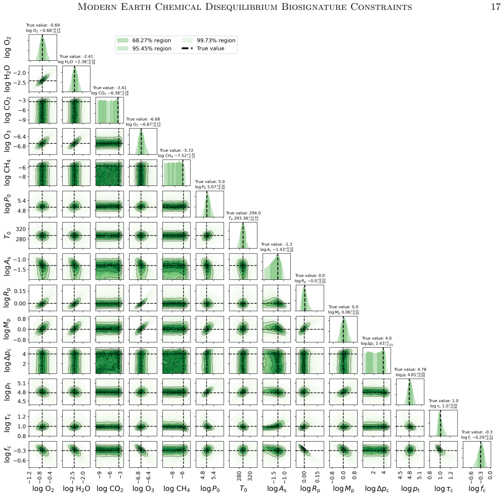
- [Section 2.3, Figure 2] The AGFE posterior is built by "randomly sampling the marginal posterior distributions" of P0, T0, O2, H2O, CO2, O3, and CH4. This is equivalent to drawing from the product of seven one-dimensional marginals, which equals the joint posterior only if the parameters are independent. The paper does not establish independence: the appendix corner plots (Figures 12-17) are the natural diagnostic, but no covariance summary or independence test is reported, and correlations are plausible (e.g., CH4 and T0 both affect overlapping water/methane features; Section 3.2 already reports profile-induced biases in P0 and O3). Because every AGFE posterior in Figures 7 and 10 is produced through this step, the central quantitative claims—CH4-limited AGFE detection for reflected light at SNRs 10-40, and tight AGFE only at 1-2 ppm transit noise with loss at 5 ppm—are not robust until the propagation is repeated with draws from the joint MCMC posterior or the independence assumption is explicitly validated. The independent-marginal scheme also risks generating unphysical parameter combinations, such as mixing ratios summing above unity; the manuscript does not describe any rejection or constraint applied during the N2 back-fill.
- [Section 3.2, Eq. (4)] The reflected-light retrieval adopts isothermal, constant-mixing-ratio profiles while the synthetic data are generated from altitude-dependent Atmos profiles. The authors show that this assumption biases P0 substantially high (about an order of magnitude in Section 3.2; a factor of 5 in Section 4) and biases O3 relative to the column average. They assert that these parameters have a negligible effect on the AGFE, but no sensitivity test is provided. Since Eq. (4) contains an explicit pressure term, RU T ln(NiP/NP°), a quantitative check—for example, propagating the constant-profile control retrieval (Figure 11) through the thermodynamics model, or recomputing the AGFE with the biased P0—is needed to separate the claimed low-bias AGFE result from retrieval-systematics effects.
minor comments (5)
- [Section 2.1] Equations (1)-(3) mix scalar and vector notation in a way that is hard to follow; a short notation table would improve reproducibility.
- [Section 3.2] The text says observations have "constant noise specified at V-band," while Section 2.1 says the noise model simulates "constant signal-to-noise along the full wavelength range"; these statements should be reconciled.
- [Section 4] The calculation of the SNR 192 requirement for a CH4 detection is not described; the readership cannot reproduce this number without the spectral-differencing formula and the assumed noise scaling.
- [Figures 7 and 10] The AGFE posterior distributions should be summarized numerically (median and credible interval) in the text or captions, since the visual histograms alone do not support the stated "tight" versus "unconstrained" thresholds.
- [General] Several typographical and wording issues remain, including "Therfastretrieval model" in Section 2.1, "affect" for "effect" in Section 3.2, and "repoted" in Section 4.
Circularity Check
No significant circularity: the AGFE posteriors are obtained by propagating retrieval posteriors through a published thermodynamics model, and no target quantity is used as a fitted input.
full rationale
This paper is an injection-recovery study: the rfast forward model generates synthetic reflected-light and transit spectra, the retrieval framework recovers atmospheric parameters, and the thermodynamics model converts those retrieved parameters into posterior distributions for the available Gibbs free energy (AGFE). No free constant is fitted to the AGFE values themselves, and the reported detectability conclusions follow from the widths and biases of the retrieval posteriors rather than from any input that already encodes the answer. The AGFE metric is taken from Krissansen-Totton et al. (2016), a prior paper that includes a co-author of the present work, but that metric is an externally published thermodynamic definition and is not redefined by the retrieval outputs; citing it is legitimate support, not circularity. Similarly, the rfast retrieval code originates in Robinson & Salvador (2023), co-authored by another author of this paper, but it is public software with an established forward model and is not used to force the target result. The main methodological concern, noted in Section 2.3 and Figure 2, is that the coupled model randomly samples the marginal posterior distributions of O2, CH4, H2O, CO2, O3, P0, and T0 and treats the product of marginals as the joint posterior for AGFE propagation. If these parameters are correlated, the resulting AGFE distribution could be too narrow or incorrectly centered. This is a statistical validity risk rather than circularity, because the output is not equivalent to the input by construction; it is a propagation approximation. Overall, the derivation chain is self-contained against its stated inputs, and the self-citations are to prior methods and metrics that carry independent content.
Assumptions & free parameters
assumptions (5)
- domain assumption rfast radiative transfer and noise models accurately represent reflected-light and transit spectra of Earth-like atmospheres.
- domain assumption Available Gibbs free energy, computed with the Krissansen-Totton et al. (2016) thermodynamics model, is a valid remote metric for chemical disequilibrium.
- domain assumption Gas-phase only AGFE, with ocean and multiphase contributions excluded, is a conservative and adequate measure for remote sensing.
- domain assumption Retrieval forward models with isothermal and constant mixing ratio profiles are adequate for the simulated observations.
- ad hoc to paper Independently sampling marginal posteriors is equivalent to sampling the joint posterior when propagating to AGFE.
Cite this review
Pith. "Pith review of Modern Earth-like Chemical Disequilibrium Biosignatures Are Challenging To Constrain Through Spectroscopic Retrievals." pith.science (2026). https://pith.science/paper/LUL2ODPI
@misc{pith2026250516231,
  author       = {Pith},
  title        = {Pith review of: Modern Earth-like Chemical Disequilibrium Biosignatures Are Challenging To Constrain Through Spectroscopic Retrievals},
  year         = {2026},
  howpublished = {\url{https://pith.science/paper/LUL2ODPI}},
  note         = {Machine review of arXiv:2505.16231}
}
read the original abstract
Robust exoplanet characterization studies are underway, and the community is looking ahead toward developing observational strategies to search for life beyond our solar system. With the development of life detection approaches like searching for atmospheric chemical species indicative of life, chemical disequilibrium has also been proposed as a potentially key signature for life. Chemical disequilibrium can arise from the production of waste gases due to biological processes and can be quantified using a metric known as the available Gibbs free energy. The main goal of this study was to explore the detectability of chemical disequilibrium for a modern Earth-like analog. Atmospheric retrievals coupled to a thermodynamics model were used to determine posterior distributions for the available Gibbs free energy given simulated observations at various noise levels. In reflected light, chemical disequilibrium signals were difficult to detect and limited by the constraints on the CH4 abundance, which was challenging to constrain for a modern Earth case with simulated observations spanning ultraviolet through near-infrared wavelengths with V-band SNRs of 10, 20, and 40. For a modern Earth analog orbiting a late-type M dwarf, we simulated transit observations with the James Webb Space Telescope Mid-Infrared Instrument (MIRI) and found that tight constraints on the available Gibbs free energy can be achieved, but only at extremely low noise on the order of several ppm. This study serves as further proof of concept for remotely inferring chemical disequilibrium biosignatures and should be included in continuing to build life detection strategies for future exoplanet characterization missions.
Figures


Figures from the paper (14 more)




Reference graph
Works this paper leans on
-
[1]
Arney, G., Domagal-Goldman, S. D., Meadows, V. S., et al. 2016, Astrobiology, 16, 873, doi: 10.1089/ast.2015.1422
arXiv 2016
-
[2]
Arney, G. N. 2019, Astrophysical Journal Letters, 873, L7, doi: 10.3847/2041-8213/ab0651
-
[3]
Arney, G. N., Meadows, V. S., Domagal-Goldman, S. D., et al. 2017, The Astrophysical Journal, 836, 49, doi: 10.3847/1538-4357/836/1/49
-
[4]
K., Changeat, Q., Garland, R., et al
Barstow, J. K., Changeat, Q., Garland, R., et al. 2020, Monthly Notices of the RAS, 493, 4884, doi: 10.1093/mnras/staa548
-
[5]
2012, Astrophysical Journal, 753, 100, doi: 10.1088/0004-637X/753/2/100
Benneke, B., & Seager, S. 2012, Astrophysical Journal, 753, 100, doi: 10.1088/0004-637X/753/2/100
-
[6]
J., Koch, D., Basri, G., et al
Borucki, W. J., Koch, D., Basri, G., et al. 2010, Science, 327, 977 24Young et al
work page 2010
-
[7]
Cubillos, P., Harrington, J., Loredo, T. J., et al. 2017, Astronomical Journal, 153, 3, doi: 10.3847/1538-3881/153/1/3
-
[8]
Dressing, C. D., & Charbonneau, D. 2013, The Astrophysical Journal, 767, 95, doi: 10.1088/0004-637X/767/1/95
Show all 44 references
-
[9]
2019, Thermodynamics, Statistical Thermodynamics, and Kinetics, 4th edn
Engel, T., & Reid, P. 2019, Thermodynamics, Statistical Thermodynamics, and Kinetics, 4th edn. (New York: Pearson Education)
2019
-
[10]
J., Villanueva, G
Fauchez, T. J., Villanueva, G. L., Schwieterman, E. W., et al. 2020, Nature Astronomy, 4, 372, doi: 10.1038/s41550-019-0977-7
2020 doi
-
[11]
K., Robinson, T
Feng, Y. K., Robinson, T. D., Fortney, J. J., et al. 2018, Astronomical Journal, 155, 200, doi: 10.3847/1538-3881/aab95c
2018 doi
-
[12]
W., Lang, D., & Goodman, J
Foreman-Mackey, D., Hogg, D. W., Lang, D., & Goodman, J. 2013, Publications of the Astronomical Society of the Pacific, 125, 306, doi: 10.1086/670067
2013 doi
-
[13]
S., Seager, S., Mennesson, B., et al
Gaudi, B. S., Seager, S., Mennesson, B., et al. 2018, Nature Astronomy, 2, 600, doi: 10.1038/s41550-018-0549-2
2018 doi
-
[14]
P., Line, M
Greene, T. P., Line, M. R., Montero, C., et al. 2016, The Astrophysical Journal, 817, 17, doi: 10.3847/0004-637X/817/1/17
2016 doi
-
[15]
R., & Lovelock, J
Hitchcock, D. R., & Lovelock, J. E. 1967, Icarus, 7, 149, doi: 10.1016/0019-1035(67)90059-0
1967 doi
-
[16]
M., & Buchhave, L
Kozakis, T., Mendon¸ ca, J. M., & Buchhave, L. A. 2022, Astronomy & Astrophysics, 665, A156, doi: 10.1051/0004-6361/202244164
2022 doi
-
[17]
S., & Catling, D
Krissansen-Totton, J., Bergsman, D. S., & Catling, D. C. 2016, Astrobiology, 16, 39, doi: 10.1089/ast.2015.1327
2016
-
[18]
Krissansen-Totton, J., Garland, R., Irwin, P., & Catling, D. C. 2018a, Astronomical Journal, 156, 114, doi: 10.3847/1538-3881/aad564
-
[19]
Krissansen-Totton, J., Olson, S., & Catling, D. C. 2018b, Science Advances, 4, eaao5747, doi: 10.1126/sciadv.aao5747
-
[20]
R., Wolf, A
Line, M. R., Wolf, A. S., Zhang, X., et al. 2013, Astrophysical Journal, 775, 137, doi: 10.1088/0004-637X/775/2/137
2013 doi
-
[21]
1975, Proceedings of the Royal Society of London
Lovelock, J. 1975, Proceedings of the Royal Society of London. Series B. Biological Sciences, 189, 167, doi: 10.1098/rspb.1975.0051
1975
-
[22]
Lovelock, J. E. 1965, Nature, 207, 568, doi: 10.1038/207568a0
1965 doi
-
[23]
E., Marley, M
Lupu, R. E., Marley, M. S., Lewis, N., et al. 2016, Astronomical Journal, 152, 217, doi: 10.3847/0004-6256/152/6/217
2016 doi
-
[24]
S., & Lincowski, A
Lustig-Yaeger, J., Meadows, V. S., & Lincowski, A. P. 2019, Astrophysical Journal, 158, 27, doi: 10.3847/1538-3881/ab21e0
2019 doi
-
[25]
J., & Batalha, N
MacDonald, R. J., & Batalha, N. E. 2023, Research Notes of the American Astronomical Society, 7, 54, doi: 10.3847/2515-5172/acc46a
2023 doi
-
[26]
2009, The Astrophysical Journal, 707, 24, doi: 10.1088/0004-637X/707/1/24
Madhusudhan, N., & Seager, S. 2009, The Astrophysical Journal, 707, 24, doi: 10.1088/0004-637X/707/1/24
2009 doi
-
[27]
Meadows, V. S. 2017, Astrobiology, 17, 1022, doi: 10.1089/ast.2016.1578
2017
-
[28]
S., Reinhard, C
Meadows, V. S., Reinhard, C. T., Arney, G. N., et al. 2018, Astrobiology, 18, 630, doi: 10.1089/ast.2017.1727
2018
-
[29]
2023, The Astrophysical Journal, 165, 265, doi: 10.3847/1538-3881/acd175
Ment, K., & Charbonneau, D. 2023, The Astrophysical Journal, 165, 265, doi: 10.3847/1538-3881/acd175
2023 doi
-
[30]
A., Howard, A
Petigura, E. A., Howard, A. W., & Marcy, G. W. 2013, Proceedings of the National Academy of Science, 110, 19273, doi: 10.1073/pnas.1319909110
2013 doi
-
[31]
D., & Kopparapu, R
Domagal-Goldman, S. D., & Kopparapu, R. K. 2020, The Astrophysical Journal Letters, 898, L33, doi: 10.3847/2041-8213/aba4a1
2020 doi
-
[32]
R., Winn, J
Ricker, G. R., Winn, J. N., Vanderspek, R., et al. 2015, Journal of Astronomical Telescopes, Instruments, and Systems, 1, 014003
2015
-
[33]
Roberge, A., & Moustakas, L. A. 2018, Nature Astronomy, 2, 605, doi: 10.1038/s41550-018-0543-8
2018 doi
-
[34]
Robinson, T. D. 2017, The Astrophysical Journal, 836, 236, doi: 10.3847/1538-4357/aa5ea8
2017 doi
-
[35]
D., & Salvador, A
Robinson, T. D., & Salvador, A. 2023, The Planetary Science Journal, 4, 10, doi: 10.3847/PSJ/acac9a
2023 doi
-
[36]
2015, Astrophysical Journal, 806, 137, doi: 10.1088/0004-637X/806/1/137
Rugheimer, S., Segura, A., Kaltenegger, L., & Sasselov, D. 2015, Astrophysical Journal, 806, 137, doi: 10.1088/0004-637X/806/1/137
2015 doi
-
[37]
K., Liu, R., & Wang, A
Rustamkulov, Z., Sing, D. K., Liu, R., & Wang, A. 2022, The Astrophysical Journal Letters, 928, L7, doi: 10.3847/2041-8213/ac5b6f
2022 doi
-
[38]
1993, Nature, 365, 715, doi: 10.1038/365715a0
Hord, C. 1993, Nature, 365, 715, doi: 10.1038/365715a0
1993 doi
-
[39]
W., Kiang, N
Schwieterman, E. W., Kiang, N. Y., Parenteau, M. N., et al. 2018, Astrobiology, 18, 663, doi: 10.1089/ast.2017.1729
2018
-
[40]
F., Meadows, V., et al
Segura, A., Kasting, J. F., Meadows, V., et al. 2005, Astrobiology, 5, 706, doi: 10.1089/ast.2005.5.706
2005 doi
-
[41]
2013, Earth System Dynamics, 4, 317, doi: 10.5194/esd-4-317-201310.5194/esdd-3-1287-2012
Simoncini, E., Virgo, N., & Kleidon, A. 2013, Earth System Dynamics, 4, 317, doi: 10.5194/esd-4-317-201310.5194/esdd-3-1287-2012
2013 arXiv
-
[42]
2022, The Astrophysical Journal, 927, 90, doi: 10.3847/1538-4357/ac4d99
Youngblood, A., & Arney, G. 2022, The Astrophysical Journal, 927, 90, doi: 10.3847/1538-4357/ac4d99
2022 doi
-
[43]
L., et al
Wunderlich, F., Godolt, M., Grenfell, J. L., et al. 2019, Astronomy and Astrophysics, 624, A49, doi: 10.1051/0004-6361/201834504 Modern Earth Chemical Disequilibrium Biosignature Constraints25
2019 doi
-
[44]
V., Robinson, T
Young, A. V., Robinson, T. D., Krissansen-Totton, J., et al. 2024, Nature Astronomy, 8, 101, doi: 10.1038/s41550-023-02145-z
2024 doi
Reviewed August 7, 2026 · model on record in the stance chip above.
Discussion (0). Continue with ORCID to comment.