Generalized random matrix model with additional interactions

Dong Wang; K. A. Muttalib; Kazi Alam; Swapnil Yadav

REVIEW 5 major objections 5 minor 18 references

Generalized random matrix model with additional interactions

T0 review · 5 major / 5 minor · reviewed 2026-08-14 · deepseek-v4-flash

Challenge this review Re-run · record.json Download PDF Read on arXiv ↗ Review JSON

Pith's one-line read The paper shows that a log-gas with an added two-body interaction is equivalent, for its equilibrium density, to a standard ensemble with a gamma-dependent effective potential.

desk verdict A plausible numerical extension of the Claeys–Romano method to a γ-deformed Muttalib–Borodin ensemble, but the effective-potential equivalence rests on an unproven one-cut assumption and needs a consistency check before I'd fully trust it. read the letter →

arxiv 1908.03726 v2 pith:M2KWOIYH submitted 2019-08-10 cond-mat.dis-nn math-phmath.MP

Swapnil Yadav , Kazi Alam , K. A. Muttalib , Dong Wang This is my paper · ORCID

classification cond-mat.dis-nnmath-phmath.MP MSC 60B2082B44

keywords gamma-ensemblelog-gasmodelrandommatrixensembleRiemann-HilbertproblemJoukowskytransformeffectiveconfiningpotentialhard-edgedensityexponentdisorderedconductors

verification ladder T0 review T1 audit T2 compute T3 formal

The pith

A machine-rendered reading of the paper's core claim, the machinery that carries it, and where it could break.

The reading

The paper introduces a log-gas model, the $\gamma$-ensemble, where a parameter $\gamma$ controls the strength of a second two-body interaction on top of the usual logarithmic repulsion. Its central claim is that, despite this extra interaction, the equilibrium density is exactly that of the known $\gamma=1$ ensemble, provided the confining potential is replaced by a $\gamma$-dependent effective potential. The effective potential is obtained by solving a self-consistent linear integral equation, and the authors implement this numerically for a linear confining potential and for an exponential interaction. The main quantitative result is that the power-law divergence of the density at the hard edge changes continuously from $-1/3$ at $\gamma=1$ to $-1/2$ at $\gamma=0$. A reader would care because this provides a solvable interpolation between two known random-matrix limits and a concrete tool for interaction-strength crossovers.

What carries the argument

The central objects are the vector-valued Riemann-Hilbert problem for the transforms $g$ and $\tilde g$ and the Joukowsky transform $J_c(s)=c(s+1)(s+1/s)^{1/\theta}$, which maps a contour $\nu$ in the $s$-plane onto the cut plane of the density. The technical step is to encode the $\gamma$ modification in a function $f(x;\gamma)$, defined so that $V'_{\mathrm{eff}}=f/x$, and to convert the Riemann-Hilbert data into the linear integral equation (25) for $f$. This $f$ fixes the endpoint parameter $c$ through Eq. (20) and the density through Eq. (29), reducing the $\gamma$-ensemble to an effective one-body problem.

What would settle it

Compute the equilibrium density for $\theta=2$, $V=2x$, and a representative $\gamma$ such as $0.5$ by an independent numerical method (direct minimization of the energy functional or Monte Carlo sampling of the log-gas) and compare the support and density profile with the integral-equation solution. If the support has more than one component, or the near-zero density exponent differs from the computed value, the effective-potential claim fails for that $\gamma$.

Watch

Extended reading notes

Core claim

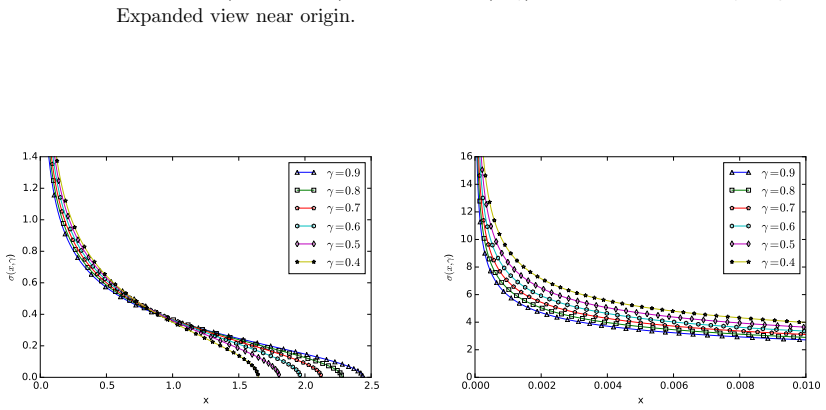
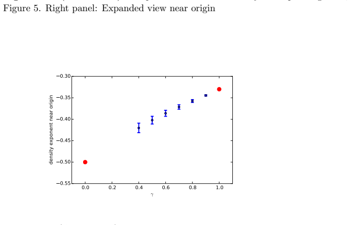
For $0<\gamma\le 1$, the joint density of Eq. (4) has an equilibrium measure whose support is taken to be a single interval $[0,b]$ with a hard edge. Within this one-cut regime, the vector-valued Riemann-Hilbert problem of the $\gamma=1$ case still governs the problem, with the $\gamma$ dependence entering through a function $f(x;\gamma)$. Defining the effective potential by $V'_{\mathrm{eff}}(x;\gamma)=f(x;\gamma)/x$, the function $f$ obeys the linear integral equation (25), whose kernel is built from the inverse of the Joukowsky transform. Solving this equation self-consistently with the endpoint condition (20) yields the equilibrium density through formula (29). For the worked example $V=2x$, $\theta=2$, the computed density shows the hard-edge exponent crossing continuously from $-1/3$ at $\gamma=1$ to $-1/2$ at $\gamma=0$; the same scheme, with the appropriate Joukowsky transform, is applied to an exponential interaction on the whole real line, where the density has two soft edges and stays non-diverging while the effective potential varies with $\gamma$.

Load-bearing premise

The construction assumes the equilibrium measure is supported on a single interval $[0,b]$ for every $0<\gamma\le 1$; if the support splits into multiple intervals, the single-contour Joukowsky transform and the integral equation no longer apply.

Editorial extensions

If this is right

For any $\gamma$ in $(0,1]$, the equilibrium density of the $\gamma$-ensemble can be computed by solving a single linear integral equation, once the inverse Joukowsky map is known.
The hard-edge exponent is not fixed by the exponent $\theta$ alone; it varies continuously with the interaction strength $\gamma$, interpolating between the $\gamma=1$ and $\gamma=0$ limits.
The effective-potential picture means existing techniques for the $\gamma=1$ ensemble, including correlation kernels, can in principle be adapted to the $\gamma$-ensemble.
The method is not specific to power-law interactions: the same construction works for an exponential interaction $r(x)=e^x$, giving non-diverging densities with $\gamma$-dependent effective potentials.
The $\gamma=0$ limit connects to the known orthogonal-Laguerre behavior with hard-edge exponent $-1/2$.

Reading between the lines

Editorial extensions of the paper, not claims the author makes directly.

If the effective-potential mapping extends beyond the one-point density to correlation kernels, the $\gamma$-ensemble would inherit the integrable structure of the $\gamma=1$ ensemble; this is a testable extension the paper leaves open.
The one-cut assumption may fail for some $\gamma$ near $0$ or for other confining potentials, producing a multi-cut support; a numerical scan of the support as a function of $\gamma$ would delimit where the construction is valid.
The same integral-equation method could be applied to other monotone functions $r(x)$ to test whether the $\gamma=0$ hard-edge exponent is always $-1/2$ or depends on the form of the interaction.
The crossover curve of the exponent in Fig. 7 invites a scaling-law fit, which could expose a universal interpolation between the two known limits.

Share X Bluesky LinkedIn Reddit HN

Signed reviews

No signed human review yet.

Editorial analysis

A structured set of objections, weighed in public.

Desk editor's note, referee report, and a circularity audit.

Desk Editor's Note

read the letter

Fair warning before you read: this is a numerical extension of Claeys–Romano to a γ-parameter family of log-gases, and the headline claim—that the γ-ensemble is an MB ensemble with an effective potential—is plausible but rests on an unproven one-cut assumption. I don't think it's wrong, and it deserves a real referee, but it needs work before I'd trust the central equivalence.

What's genuinely new: the model in Eq. (4) is a natural generalization of Muttalib–Borodin with a tunable exponent γ on the second interaction, motivated by the quasi-1D to 3D crossover in disordered conductors. The adaptation of the CR Riemann–Hilbert machinery to 0<γ<1 is real, and the numerical method gives a concrete way to compute densities for this family. The endpoint checks are honest: γ=1 recovers MB, and the hard-edge exponent goes from −1/3 to −1/2 as γ→0, matching the known Laguerre limit. That's a nontrivial sanity check, and I believe it. The extension to r(x)=e^x is a nice bonus that shows the technique isn't tied to the x^θ interaction. Citations look appropriate: CR, CW, Borodin, Forrester, and the Muttalib–Gopar–Wölfle line are the relevant anchors.

Soft spots, in order of severity. First, the one-cut assumption. The whole construction uses a single contour ν and a two-preimage relation on [0,b]. For γ<1 there is no proof—and as far as I can tell no numerical check—that the equilibrium measure stays supported on one interval. If the support splits, the integral equation (25) solves a different model from the original γ-ensemble. This is load-bearing, because the effective-potential equivalence is exactly an equality of equilibrium measures. Second, equation (12) is asserted rather than derived; it's the generalized jump condition that drives everything. A direct Euler–Lagrange consistency check—plug the computed density back into (6)—would catch a wrong jump condition, and I'd want to see that in the paper. Third, the numerics are under-described: no discretization scheme, no convergence test, no error analysis, and no code. Figure 7 has error bars, but I can't reproduce the method from the text as it stands. Finally, the abstract and summary overclaim: "any two-body interaction" with a known Joukowsky transform is too broad, and the effective-potential picture is more a reformulation than a predictive mapping. That's not circularity, but it's not an independent check either.

Who gets value: people working on log-gas/RH methods and mesoscopic transport toy models. This is a serious paper, not a desk reject. I'd send it to peer review, but with a strong request for a one-cut proof or numerical evidence, a derivation or consistency verification of (12), and proper numerical details.

Referee Report

5 major / 5 minor

Summary. The paper introduces a log-gas model (4), the 'γ-ensemble', whose joint density contains the additional two-body factor |x_i^θ - x_j^θ|^γ on the non-negative half-line. The authors adapt the Claeys-Romano (CR) Riemann-Hilbert method for the Muttalib-Borodin ensemble to derive an integral equation (25) for an auxiliary function f, define an effective potential Veff by Veff' = f/x, and claim that the γ-ensemble is equivalent at the level of the global equilibrium density to an MB ensemble with potential Veff. For V(x)=2x and θ=2, they compute the hard-edge density and report a crossover of the edge exponent from -1/3 at γ=1 to -1/2 at γ=0 (Figure 7). A second example with r(x)=e^x and V=x^2/2 is treated in Section 6 and the Appendix. The main difficulties are that the one-cut support assumption is unproven for γ<1, the derivation of the integral equation contains a visible typo in Eq. (24), the numerical solution is undocumented, and the density formula (29) contains a factor 1/γ that appears inconsistent with the claimed MB mapping.

Significance. If correct, the effective-potential mapping is a useful simplification: it reduces the two-body interaction with strength γ to a one-body confining potential, and the hard-edge exponent crossover is a concrete quantitative prediction that can be tested by independent numerical simulation of the log-gas (4). The paper builds on a rigorous framework (CR) and treats both hard-edge and soft-edge examples, with the γ=0 and γ=1 limits matching known ensembles, which is a good sanity check. However, the central equivalence is not yet established: the one-cut assumption is load-bearing and unchecked, the derivation has gaps and typos, and the numerical evidence lacks reproducibility details. The approach is promising, but the manuscript needs substantial revision before the claims can be accepted.

major comments (5)

[Section 3] The entire construction for 0<γ<1 presupposes that the equilibrium measure of (4) is supported on a single interval [0,b] with a hard edge at 0 and no interior gaps, but this one-cut condition is only stated for γ=1 in Section 2 and is neither proved nor numerically checked for γ<1. The Joukowsky transform (10), the contour ν, and the two-preimage relation Jc(s1)=Jc(s2)=x all depend on this geometry; if the support develops a gap or splits as γ varies, equation (25) solves a different model from the original γ-ensemble. I do not object to the generalized jump condition (12), which does follow from (13) and the Euler-Lagrange equation (6), but the unproven one-cut assumption is load-bearing for the claimed equivalence and needs a proof or at least a numerical test that the computed density satisfies (6) on [0,b] and the variational inequality outside.
[Section 4, Eq. (29)] Equation (29) contains an explicit factor 1/γ in front of the integral, while the CR formula for the MB ensemble (γ=1) has no such factor. As written, the γ-ensemble density is (1/γ) times the MB density with effective potential Veff, so the statement that 'the density for γ<1 has the same expression as that for γ=1, except that V is replaced by Veff' is not literally correct; moreover, if both densities are normalized to 1, such a constant factor cannot be right. Please reconcile the factor with the effective-potential mapping and show that the raw output of (29) integrates to 1 without an ad hoc normalization.
[Section 3, Eq. (24)] The two formulas displayed for N+(s1) and N-(s2) in Eq. (24) are identical, which must be a typo; the kernel φ in Eq. (26) indicates that the second line should involve \bar h(y) in the denominators. As printed, the derivation of the integral equation (25) cannot be followed. Please correct Eq. (24) and include the intermediate steps that lead to (25), including the contour orientations and the branch choices for h and \bar h.
[Section 5] The numerical solution is not documented: the paper states that (25) and (20) are solved self-consistently but gives no discretization scheme, quadrature rule, iteration procedure, convergence criterion, or error analysis. Figure 7 reports 'uncertainties in the numerical estimates' but the source of these uncertainties is not explained. Without this information, the central numerical prediction (the exponent crossover) is not reproducible and the quoted exponents cannot be assessed.
[Appendix, Eq. (39)] The soft-edge integral equation (39) differs from the hard-edge equation (25) by the absence of the constant term, and the density formula (44) has no 1/γ factor whereas (29) does. If both cases are meant to follow from the same effective-potential construction, the structural difference should be explained; otherwise the presence/absence of the 1/γ factor looks like an inconsistency rather than a feature of the different boundary conditions.

minor comments (5)

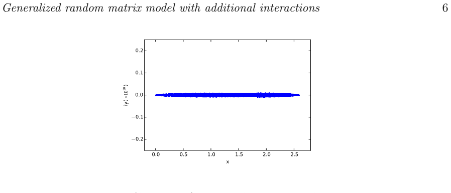
[Figures 2 and 11] The y-axis label 'iy(×10^{10})' is unclear; the text says the tiny imaginary parts are numerical noise. Please relabel the axis as Im(Jc(s)) and state whether the plotted curve is the raw numerical map or a smoothed curve.
[Figure 6 caption] The caption says 'Normalized density'; please specify how the normalization is performed and whether Eq. (29) was already normalized or was rescaled for display.
[Equations (23)-(26)] The inverse map h is double-valued; the paper uses h(x) and \bar h(x) without defining which preimage is h(x) and without stating that \bar h is the complex conjugate branch. Please define the branches precisely.
[Abstract and Section 1] The abstract says the density is computed by 'numerically solving the Riemann-Hilbert problem'; in fact the paper solves a scalar integral equation obtained after assuming an RH reduction. Please rephrase to match the actual method.
[Equation (6)] The Euler-Lagrange equation is written with V(x) on the left and the constant l on the right; in Eq. (9a) the constant appears as V(x)+l. Please unify the sign convention.

Circularity Check

0 steps flagged · score 0.0 of 10

No circular derivation found: the effective potential is a reformulation of the solved equilibrium equations, not a fitted or imported input.

full rationale

The paper's central derivation is a self-contained RH/integral-equation calculation. The function f(x;γ) is obtained by solving the integral equation (25) together with the normalization condition (20) for the Joukowsky parameter c; these equations come from the Euler-Lagrange conditions of the γ-ensemble equilibrium problem, not from any preset density. The effective potential Veff is then introduced by the definition V′eff(x;γ)=f(x;γ)/x in Eq. (27), and the density formula (29) is derived from the same RH solution. Thus the statement that the γ-ensemble can be represented as an MB ensemble with an effective potential is a post-hoc mathematical reformulation of the solved equations, not an independent prediction that has been assumed as input. The hard-edge exponent crossover in Fig. 7 is computed from this solution, with the γ=1 and γ=0 points used only as analytic consistency checks, so no fitted parameter is being relabeled as a prediction. The paper does rely on the one-cut hard-edge support assumption for 0<γ<1, carried over from Claeys-Romano without a proof, but this is an unverified modeling assumption and a correctness risk rather than a circular step: the derivation does not assume the final density or the final exponent. Self-citations to CR and CW provide the Joukowsky transformation and the γ=1 RH setup, which are explicit mathematical inputs stated in the paper (e.g., Eq. (10) and Eq. (32)); CW's JT is given explicitly and is independently checkable even though one author overlaps. These citations are not used to forbid alternatives or to smuggle in the target result. Accordingly, no load-bearing circularity is exhibited, and the appropriate score is 0.

Assumptions & free parameters 0 free parameters · 4 assumptions · 0 invented entities

The central claim rests on the one-cut support assumption, the validity of the generalized RH jump condition, the existence and uniqueness of the numerical integral equation solution, and the analytic properties of the Joukowsky transform. None of these are proved for γ<1 in the paper, though the endpoint checks at γ=1 and γ=0 are reassuring. No free parameters are fitted to external data, and no new entities are introduced.

assumptions (4)

domain assumption The equilibrium measure for the γ-ensemble remains supported on a single interval [0,b] with a hard edge for all 0<γ≤1.
This one-cut condition is invoked when setting up the RH problem with a single Joukowsky transform after Eq. (6). For γ=1 it is a theorem in CR [17], but for γ<1 no proof is given.
domain assumption The vector RH problem of Section 2, with property (9a) replaced by (12), fully characterizes the equilibrium measure for γ<1.
The paper states 'our g and g̃ satisfy the RH problem' but does not prove the generalized jump condition (12) beyond writing it down; the derivation is heuristic.
domain assumption The Joukowsky transformation (10) and its inverse h(x) have the same analytic properties on and inside the contour ν for all γ in (0,1] as in the γ=1 case.
The JT itself is independent of γ, but the contour and inverse mapping properties are only verified numerically in Figures 1-3; no analytic proof is given for γ<1.
domain assumption The nonlinear integral equation (25) for f, together with the normalization condition (20), has a unique solution and the numerical iteration converges to it.
No existence, uniqueness, or convergence analysis is provided. The paper reports only that the equations are solved 'numerically self-consistently'.

how reviews work

0 comments

Cite this review

Pith. "Pith review of Generalized random matrix model with additional interactions." pith.science (2026). https://pith.science/paper/M2KWOIYH

@misc{pith2026190803726,
  author       = {Pith},
  title        = {Pith review of: Generalized random matrix model with additional interactions},
  year         = {2026},
  howpublished = {\url{https://pith.science/paper/M2KWOIYH}},
  note         = {Machine review of arXiv:1908.03726}
}

abstract

We introduce a log-gas model that is a generalization of a random matrix ensemble with an additional interaction, whose strength depends on a parameter $\gamma$. The equilibrium density is computed by numerically solving the Riemann-Hilbert problem associated with the ensemble. The effect of the additional parameter $\gamma$ associated with the two-body interaction can be understood in terms of an effective $\gamma$-dependent single-particle confining potential.

Figures

Figures reproduced from arXiv: 1908.03726 by the authors.

**Figure 1.** (Color online) ν contour for θ = 2, c = 1. 3. Effective potential To accommodate 0 < γ < 1 for non-negative eigenvalues within the CR framework, we consider the hard edge case, focusing on θ = 2 for simplicity. A closer look of the JT for hard edge (10) shows that it is analytic in C\[−1, 0] and has critical points on real line at Sa = −1 and Sb = 1 θ which are mapped to points 0 and b, respectively. There also exis… view at source ↗

**Figure 2.** (Color online) Mapping for ν1 contour, θ = 2, c = 1. Mapping for ν2 looks similar. (1) (2) (5) (6) (3) (4) g D ~ (3) (2) + g ~ 0 J :D\[−1,0] H \[0,b] c θ g+ g− (1) (4) 0 S b b J :C\D C\[0,b] c 0 (6) (5) ν1 ν 2 b − Sa [PITH_FULL_IMAGE:figures/full_fig_p006_2.png] view at source ↗

**Figure 3.** (Color online) Schematic Figure for mapping of JT, following CR. for property (9a), which is generalized to g±(x) + γg˜∓(x) − V (x) − ` = ±πi(1 − γ)µ([x, b]), (12) because for x ∈ [0, b] g±(x) = Z b 0 ln|x−y|dµ(y)±πiµ([x, b]), g˜±(x) = Z b 0 ln|x θ−y θ |dµ(y)±πiµ([x, b]). (13) Rewriting g = (1 + γ)g/2 + (1 − γ)g/2, we have that (12) is equivalent to 1 ± γ 2 g+(x) + 1 ∓ γ 2 g−(x) + γg˜∓(x) = V (x) + `. (14) F… view at source ↗

Figures from the paper (10 more)

**Figure 4.** Figure 4: (Color online) Left panel: f(x; γ) for different values of γ. Right panel: Expanded view near origin. Then the density corresponding to the γ-ensembles is computed using the relation [17] σ(y) = −[N+(s1) − N−(s2)]/2πiy. Substituting for N+(s1) and N−(s2) using Eq. (19)…

**Figure 6.** Figure 6: The diverging exponent at the hard edge changes as a function of [PITH_FULL_IMAGE:figures/full_fig_p009_6.png]

**Figure 5.** Figure 5: (Color online) Left panel: Veff(x; γ) for different values of γ. Right panel: Expanded view near origin. 0.0 0.5 1.0 1.5 2.0 2.5 x 0.0 0.2 0.4 0.6 0.8 1.0 1.2 1.4 ¾(x;°) ° =0:9 ° =0:8 ° =0:7 ° =0:6 ° =0:5 ° =0:4 0.000 0.002 0.004 0.006 0.008 0.010 x 0 2 4 6 8 10 12 14 …

**Figure 6.** Figure 6: (Color online) Left panel: Normalized density corresponding to Veff in [PITH_FULL_IMAGE:figures/full_fig_p010_6.png]

**Figure 7.** Figure 7: (Color online) Exponents with uncertainties in the numerical estimates. Points for γ = 1 and γ = 0 are known analytically [PITH_FULL_IMAGE:figures/full_fig_p010_7.png]

**Figure 8.** Figure 8: (Color online) fe(x; γ) for different values of γ. 2.0 1.5 1.0 0.5 0.0 0.5 1.0 1.5 2.0 2.5 x 0.0 0.5 1.0 1.5 2.0 2.5 3.0 3.5 4.0 Ve ff(x;°) ° =0:9 ° =0:8 ° =0:7 ° =0:6 ° =0:5 ° =0:4 2 1 0 1 2 3 x 0.0 0.1 0.2 0.3 0.4 0.5 ¾(x;°) ° =0:9 ° =0:8 ° =0:7 ° =0:6 ° =0:5 ° =0:4 …

**Figure 9.** Figure 9: (Color online) The effective potential (Left panel) and the density (Right panel) for model (31). Densities for γ = 1 and γ = 0 are known analytically. . 6. Non-diverging density Finally, as an example of a model with non-diverging density which has two soft edges, we …

**Figure 10.** Figure 10: (Color online) ν contour for c1 = 1, c0 = 0.5. 2 1 0 1 2 3 x 0.2 0.1 0.0 0.1 0.2 iy( £10 10 ) [PITH_FULL_IMAGE:figures/full_fig_p013_10.png]

**Figure 11.** Figure 11: (Color online) Mapping for ν1 contour, c1 = 1, c0 = 0.5. Mapping for ν2 looks similar. (4) (1) 𝐽𝑐1,𝑐0: ℂ\𝐷ഥ → ℂ\[a,b] a b 𝑔+(𝑥) 𝑔−(𝑥) ↓ ↑ (3) (6) (2) (5) a b ↓𝑔෤+(𝑥) ↑𝑔෤−(𝑥) 𝐽𝑐1,𝑐0:𝐷\[−1, 0] → 𝕊 \[a,b] 𝑦 = −𝑖𝜋 𝑦 = 𝑖𝜋 𝜈1 𝜈2 1 2 -1 2 (1) (2) (5) (6) (3) (4) D Sb Sa [PI…

**Figure 12.** Figure 12: (Color online) Schematic Figure for mapping of JT, following CW. conjugates of each other, such that ν1 in the upper-half plane from Sa to Sb, and a curve ν2 in the lower-half plane from Sb to Sa. We note that Jc1,c0 maps the exterior of ν to C, and the interior of ν,…

Discussion (0). Continue with ORCID to comment.

Reference graph

Works this paper leans on

18 extracted references · 17 canonical work pages

[1]

Mehta M L 2004 Random matrices 3rd ed ( Pure and Applied Mathematics (Amsterdam) vol 142) (Elsevier/Academic Press, Amsterdam) ISBN 0-12-088409-7

work page 2004
[2]

Erd˝ os L and Yau H T 2017 A dynamical approach to random matrix theory (Courant Lecture Notes in Mathematics vol 28) (Courant Institute of Mathematical Sciences, New York; American Mathematical Society, Providence, RI) ISBN 978-1-4704-3648-3

work page 2017
[3]

Forrester P J 2010 Log-gases and random matrices (London Mathematical Society Monographs Series vol 34) (Princeton, NJ: Princeton University Press) ISBN 978-0-691-12829-0

work page 2010
[4]

Beenakker C W J 1997 Rev. Mod. Phys. 69(3) 731–808 URL https://link.aps.org/doi/10. 1103/RevModPhys.69.731

work page 1997
[5]

Muttalib K A 1995 J. Phys. A 28 L159–L164 ISSN 0305-4470 URL http://stacks.iop.org/ 0305-4470/28/L159

work page 1995
[6]

B 536 704–732 ISSN 0550-3213 URL http://dx.doi.org/10

Borodin A 1999 Nuclear Phys. B 536 704–732 ISSN 0550-3213 URL http://dx.doi.org/10. 1016/S0550-3213(98)00642-7

work page 1999
[7]

Forrester P J and Wang D 2017 Electron. J. Probab. 22 Paper No. 54, 43 ISSN 1083-6489 URL https://doi-org/10.1214/17-EJP62

work page doi:10.1214/17-ejp62 2017
[8]

Zhang L 2015 J. Stat. Phys. 161 688–711 ISSN 0022-4715 URL http://dx.doi.org/10.1007/ s10955-015-1353-3

work page 2015

Show all 18 references

[9]

1088%2F1361-6544%2Fab247c

Kuijlaars A B J and Molag L D 2019 Nonlinearity 32 3023–3081 URL https://doi.org/10. 1088%2F1361-6544%2Fab247c

2019
[10]

Lueck T, Sommers H J and Zirnbauer M R 2006 J. Math. Phys. 47 103304, 24 ISSN 0022-2488 URL http://dx.doi.org/10.1063/1.2356798 Generalized random matrix model with additional interactions 16

2006 doi
[11]

Muttalib K A and Klauder J R 1999 Phys. Rev. Lett. 82(21) 4272–4275 URL https://link.aps. org/doi/10.1103/PhysRevLett.82.4272

1999 doi
[12]

Muttalib K A and Gopar V A 2002 Phys. Rev. B 66(11) 115318 URL https://link.aps.org/ doi/10.1103/PhysRevB.66.115318

2002 doi
[13]

Douglas A, Markoˇ s P and Muttalib K A 2014 J. Phys. A 47 125103, 13 ISSN 1751-8113 URL https://doi-org/10.1088/1751-8113/47/12/125103

2014 doi
[14]

Muttalib K A, Markoˇ s P and W¨ olﬂe P 2005Phys. Rev. B 72(12) 125317 URL https://link. aps.org/doi/10.1103/PhysRevB.72.125317

doi
[15]

Muttalib K A, Pichard J L and Stone A D 1987 Phys. Rev. Lett. 59(21) 2475–2478 URL https://link.aps.org/doi/10.1103/PhysRevLett.59.2475

1987 doi
[16]

Deift P A 1999 Orthogonal polynomials and random matrices: a Riemann-Hilbert approach (Courant Lecture Notes in Mathematics vol 3) (New York: New York University Courant Institute of Mathematical Sciences) ISBN 0-9658703-2-4; 0-8218-2695-6

1999
[17]

org/10.1088/0951-7715/27/10/2419

Claeys T and Romano S 2014 Nonlinearity 27 2419–2444 ISSN 0951-7715 URL http://dx.doi. org/10.1088/0951-7715/27/10/2419

2014 doi
[18]

Claeys T and Wang D 2014 Comm. Math. Phys. 328 1023–1077 ISSN 0010-3616 URL http: //dx.doi.org/10.1007/s00220-014-1988-y

2014 doi

Pith tools

Reviewed August 14, 2026 · model on record in the stance chip above.

[1] [1]

Mehta M L 2004 Random matrices 3rd ed ( Pure and Applied Mathematics (Amsterdam) vol 142) (Elsevier/Academic Press, Amsterdam) ISBN 0-12-088409-7

work page 2004

[2] [2]

Erd˝ os L and Yau H T 2017 A dynamical approach to random matrix theory (Courant Lecture Notes in Mathematics vol 28) (Courant Institute of Mathematical Sciences, New York; American Mathematical Society, Providence, RI) ISBN 978-1-4704-3648-3

work page 2017

[3] [3]

Forrester P J 2010 Log-gases and random matrices (London Mathematical Society Monographs Series vol 34) (Princeton, NJ: Princeton University Press) ISBN 978-0-691-12829-0

work page 2010

[4] [4]

Beenakker C W J 1997 Rev. Mod. Phys. 69(3) 731–808 URL https://link.aps.org/doi/10. 1103/RevModPhys.69.731

work page 1997

[5] [5]

Muttalib K A 1995 J. Phys. A 28 L159–L164 ISSN 0305-4470 URL http://stacks.iop.org/ 0305-4470/28/L159

work page 1995

[6] [6]

B 536 704–732 ISSN 0550-3213 URL http://dx.doi.org/10

Borodin A 1999 Nuclear Phys. B 536 704–732 ISSN 0550-3213 URL http://dx.doi.org/10. 1016/S0550-3213(98)00642-7

work page 1999

[7] [7]

Forrester P J and Wang D 2017 Electron. J. Probab. 22 Paper No. 54, 43 ISSN 1083-6489 URL https://doi-org/10.1214/17-EJP62

work page doi:10.1214/17-ejp62 2017

[8] [8]

Zhang L 2015 J. Stat. Phys. 161 688–711 ISSN 0022-4715 URL http://dx.doi.org/10.1007/ s10955-015-1353-3

work page 2015