On large-scale wind-drift ocean currents: An asymptotic approach in spherical coordinates

Christian Puntini; Eduard Stefanescu; Luigi Roberti

REVIEW 2 major objections 5 minor 1 cited by

On large-scale wind-drift ocean currents: An asymptotic approach in spherical coordinates

T0 review · 2 major / 5 minor · reviewed 2026-08-03 · deepseek-v4-flash

Challenge this review Re-run · record.json Download PDF Read on arXiv ↗ Review JSON

Pith's one-line read Starting from the Navier–Stokes equations in rotating spherical coordinates, this paper derives an asymptotic model for wind-driven ocean drift currents that retains full spherical geometry, proves the leading-order solution is a unique Ekm

desk verdict Nice spherical-coordinate Ekman framework with solid proofs, but the free-surface boundary condition is mis-scaled by ε, leaving the flat-surface model without a consistent asymptotic justification. read the letter →

arxiv 2602.06473 v2 pith:M6QWQ3TU submitted 2026-02-06 physics.flu-dyn math-phmath.APmath.MPphysics.ao-ph

Christian Puntini , Luigi Roberti , Eduard Stefanescu This is my paper · ORCID

classification physics.flu-dynmath-phmath.APmath.MPphysics.ao-ph MSC 35Q3035Q3576D0576U6086A05

keywords wind-drivenoceancurrentsEkmanspiralasymptoticexpansionsphericalcoordinateseddyviscositysurfacedeflectionangleRossbynumberthin-shellparameter

topics Navier-Stokes Regularity

verification ladder T0 review T1 audit T2 compute T3 formal

The pith

A machine-rendered reading of the paper's core claim, the machinery that carries it, and where it could break.

The reading

Starting from the Navier–Stokes equations in rotating spherical coordinates, the paper derives an asymptotic model for wind-driven ocean drift currents that avoids the classical tangent-plane (f-plane) approximation. The derivation uses a double expansion in two small parameters: the ratio of the Ekman depth to Earth's radius, and the Rossby number. The leading-order result is a linear complex-valued ODE for the ageostrophic current with a nonlinear wind-stress boundary condition; the paper proves this problem has a unique solution forming a classical Ekman spiral for any depth-dependent eddy viscosity. From the solution it derives a closed-form surface deflection angle, and with five explicit viscosity profiles it produces angles consistent with observed values, including both greater and less than 45°.

What carries the argument

The key object is the complex-valued boundary value problem (3.20), obtained by splitting the horizontal velocity into geostrophic and ageostrophic components after the double asymptotic expansion in the thin-shell parameter and the Rossby number. The nonlinear wind-stress boundary condition is the only nonlinearity in the leading-order problem; it is what ties the solution's amplitude to the wind. Existence and uniqueness are proved by writing W=cY with Y the solution of the linear homogeneous initial value problem, then solving a quartic for the surface-current magnitude. The surface deflection angle then follows from the complex ratio λ=Y'(0)/Y(0), giving formula (4.14) and the bounds (4.

What would settle it

At a mid-latitude site with a known, roughly depth-uniform eddy viscosity and a steady wind near 10 m/s, measure the angle between the surface current and the wind. If the observed deflection differs systematically from the value predicted by formula (4.14) with λ computed from the viscosity profile and ϱ the unique positive root of (4.8), beyond measurement uncertainty, the flat-surface leading-order model would be ruled out.

Watch

Extended reading notes

Core claim

The central claim is that the leading-order boundary value problem (m(z)W')' = 2i W sinθ, W'(0)=C|Ww−W(0)|(Ww−W(0)), W(z0)=0 has a unique solution for any positive viscosity profile m(z), and that solution is a classical Ekman spiral: its magnitude grows monotonically toward the surface and its phase rotates monotonically with depth, in the sense sign(θ)ϑ'>0. The proof reduces the nonlinear boundary condition to a fourth-order polynomial whose unique positive root fixes the surface current magnitude, and the deflection angle is then determined by the single complex number λ=Y'(0)/Y(0) associated with the linear homogeneous solution. This yields explicit deflection angles for five viscosity p

Load-bearing premise

The model assumes a flat free surface and no surface waves, so wave-induced Stokes drift and Coriolis–Stokes forcing are absent; if these wave effects materially change the near-surface momentum balance for typical winds, the predicted current directions will not correspond to the observed currents.

Editorial extensions

If this is right

The model can describe large-scale wind-drift currents without the f-plane approximation, extending Ekman theory to flows whose horizontal extent is comparable to the Earth's radius.
The surface deflection angle formula (4.14) yields predictions for any depth-dependent eddy viscosity without solving the full problem, and the bounds (4.15) approximate the angle directly from λ without solving the quartic.
For viscosity profiles decaying with depth, the model predicts deflection angles exceeding 45°, while profiles increasing with depth yield angles below 45°; the piecewise linear profile (increasing then decreasing) yields angles below 45°, suggesting the increasing part dominates.
The Ekman transport angle deviates from 45° for finite-depth layers, approaching 45° as the layer depth increases, recovering classical results in the infinite-depth limit.
The first-order correction in the Rossby number is governed by a linear problem whose solution is estimated via logarithmic matrix norms, providing a priori bounds in terms of the leading-order solution.

Reading between the lines

Editorial extensions of the paper, not claims the author makes directly.

A testable extension: the model's deflection-angle predictions could be compared against a dataset of simultaneous wind and drifter measurements stratified by latitude, wind speed and estimated eddy viscosity profile; if observed angles fall outside the range spanned by the five profiles, the flat-surface and no-Stokes-drift assumptions would be implicated.
The authors' claim that the scaling forces the vertical velocity to be order ε smaller than horizontal, thereby excluding surface waves, suggests that including a non-flat free surface would require a different scaling regime; this could be a way to incorporate Coriolis–Stokes forcing without abandoning the spherical geometry.
Since the leading-order system is essentially steady with advective time scaling, an unsteady extension with a smaller time scale would include near-inertial oscillations; the same complex-variable framework and quartic-based deflection formula may extend to that regime.

Share X Bluesky LinkedIn Reddit HN

Editorial analysis

A structured set of objections, weighed in public.

Desk editor's note, referee report, and a circularity audit.

Desk Editor's Note

read the letter

Colleague,

Read the Puntini–Roberti–Stefanescu paper. The mathematical core is real: they set up a double asymptotic expansion in the thin-shell parameter and Rossby number, derive the leading-order Ekman problem with the nonlinear wind-stress boundary condition, prove existence and uniqueness for arbitrary depth-dependent eddy viscosity, obtain deflection-angle bounds and the vanishing deflection at the equator, and give explicit Bessel-function solutions for five eddy-viscosity profiles. The proofs of Theorems 4.1 and 4.2 look correct; the polynomial argument for uniqueness is clean. This is a legitimate extension of the Constantin–Johnson spherical-coordinate program and deserves to be in the literature.

There is a problem in the derivation that the authors have missed. The non-dimensional kinematic boundary condition (2.14) is wrong by a factor of ε. From their own scaling, w' = ε U' w and h' = D' h, so both sides of the dimensional condition carry one power of ε. Dividing gives w = ∂h/∂t + u/((1+εz)cosθ)∂h/∂φ + v/(1+εz)∂h/∂θ, not εw = ... as printed. At leading order they then get an invariant condition for h0, and when they set h0 = 0, they do not impose w0 = 0 at the surface. The vertical velocity recovered from continuity is generically nonzero at z = 0 for a spatially varying wind, so the flat-surface solution violates the free-surface condition. If the flat surface is meant as a rigid lid, the pressure at the lid should be an unknown, not the imposed Ps. Either way, the asymptotic reduction is not a consistent free-surface limit. This is load-bearing for the claim that the model is derived from first principles. The ODE (3.20) might still be a good heuristic model, but the derivation needs reworking.

Other issues are minor by comparison. The statement that the results are "remarkably consistent with observations" is qualitative — the deflection-angle comparisons are visual, not a quantitative fit, and the spread across profiles is wide, so the claim is stronger than the evidence. Equation (5.20) has a spurious a_k in the coefficient; the explicit solutions don't appear to use it, but it could mislead. The abstract complaint in the reader's version (depth-varying density) does not apply to the manuscript text, which consistently says constant density.

I would send this to peer review, but I would want the authors to fix the boundary-condition scaling and either add a quantitative comparison or tone down the observational claims. The paper is worth the referees' time.

Referee Report

2 major / 5 minor

Summary. The paper derives an asymptotic model for wind-driven Ekman currents from the Navier–Stokes equations in rotating spherical coordinates, using the small thin-shell parameter ε and a small Rossby number R. The leading-order problem is reduced to the complex ODE (m(z)W')' = 2i sinθ W with a nonlinear wind-stress boundary condition at z=0 and a vanishing condition at the Ekman depth z0. The authors prove existence and uniqueness of the solution, show it forms a classical Ekman spiral, derive a formula for the surface deflection angle, and provide explicit Bessel-function solutions for five eddy-viscosity profiles. They also formulate the first-order correction in R and give a priori bounds. The central claim is that this reduced model is a consistent spherical-coordinate generalization of the classical Ekman theory and that its deflection-angle predictions agree well with observations.

Significance. If the derivation were fully consistent, the paper would be a valuable contribution: it treats a classical problem without tangent-plane approximations, gives rigorous existence/uniqueness results for a nonlinear boundary-value problem, and supplies explicit analytic solutions for several physically motivated eddy-viscosity profiles. The ODE analysis in Section 4 and the explicit computations in Section 5 appear careful and are likely correct as standalone mathematics. However, the derivation from the free-surface problem contains a scaling error in the kinematic boundary condition, which undermines the claim that (3.20) is the correct leading-order model of a flat free surface. The comparison with observations is also qualitative, since the layer depth z0 and wind magnitude |Ww| are chosen ad hoc rather than fitted systematically.

major comments (2)

[§2.3, Eq. (2.14); §3.1, Eq. (3.5)] The non-dimensional kinematic boundary condition is mis-scaled. With w' = ε U' w and h' = D' h, substituting into (2.6) gives w = ∂h/∂t + u/((1+εz)cosθ)∂h/∂φ + v/(1+εz)∂h/∂θ, not εw = .... The extra ε propagates into the expansion in §3, so (3.5) should read w0 = ∂h0/∂t + u0/cosθ ∂h0/∂φ + v0 ∂h0/∂θ on z=h0, not an invariant condition. Since the paper then sets h0=0, the correct condition would impose w0=0 at z=0. The solution obtained from (3.20) and the formula for w0 after (3.20) does not in general satisfy this, because w0(0) is determined by the horizontal divergence of the ageostrophic field. Thus the flat-surface reduction is not a consistent asymptotic limit of the free-surface problem. This is a load-bearing issue for the derivation of the central model (3.20), independent of the wave/Stokes-drift limitation acknowledged in §6. Please correct the scaling or explicitly reformulate
[§3.1 and §4, in relation to the model (3.20)] The mathematical analysis of the reduced problem (3.20) is sound, but the physical interpretation of that problem is affected by the free-surface inconsistency. If the flat surface is instead interpreted as a rigid lid, the leading-order pressure should not be fixed to the atmospheric pressure P_s; an unknown lid pressure would enter the geostrophic balance and hence alter Ww. The paper does not provide this alternative interpretation. The central claim that (3.20) is the leading-order free-surface model therefore needs either a corrected derivation or a clearly stated change of modeling assumptions.

minor comments (5)

[Abstract] The abstract states that the fluid has 'depth-varying density' and mentions 'three explicit eddy viscosity profiles,' whereas the body assumes constant density above the thermocline and actually treats five profiles. Please align the abstract with the body.
[§2.3] The parameter R = U'/(Ω'R') is called the 'inverse Rossby number,' but by the standard definition it is the Rossby number itself (up to a factor of 2 depending on convention). Please correct the terminology.
[§3.2] There is a typo: 'One more setting the coefficients to zero' should likely read 'Again setting the coefficients to zero.'
[§5.2, §5.3] The notation for the Bessel-function coefficients is inconsistent: both c2 and ec2 are used without always clarifying the relationship c2 = ec2 c1. Standardizing this notation would improve readability.
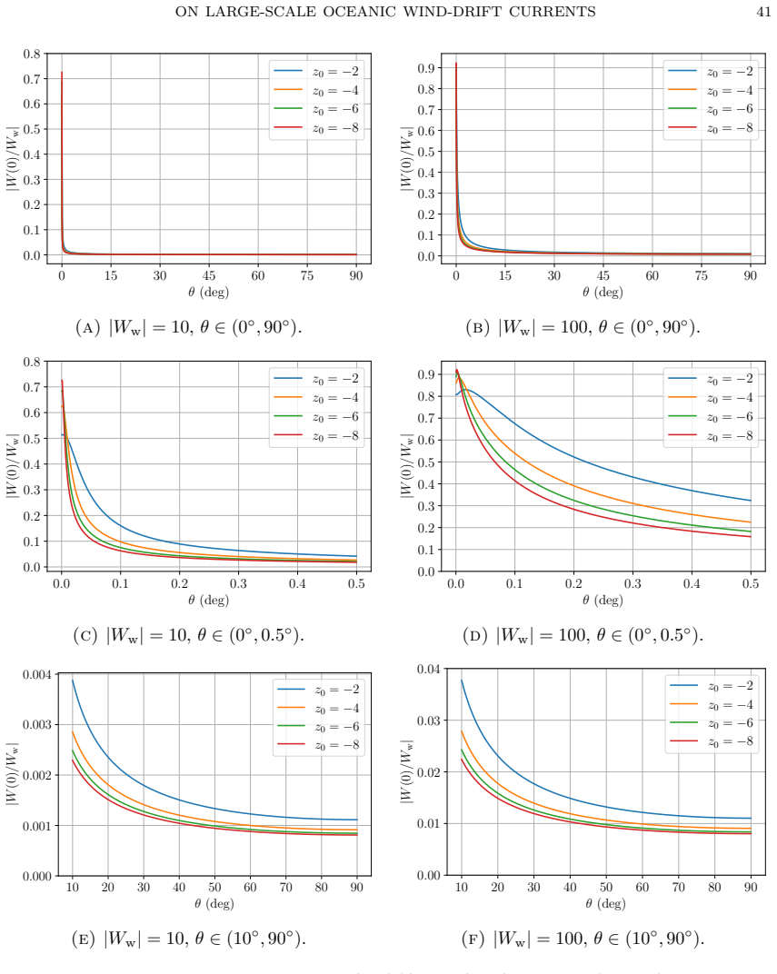
[§6] The statement that the deflection-angle results are 'remarkably consistent with observations' is somewhat strong, because z0 and |Ww| are chosen by hand in the considered ranges and no systematic comparison or uncertainty quantification is given. Please temper the claim or state explicitly that the comparison is qualitative.

Circularity Check

0 steps flagged · score 0.0 of 10

Derivation is self-contained; no circularity found.

full rationale

The paper's central derivation chain — Navier–Stokes equations (2.1), scaling (2.10), double asymptotic expansion leading to (3.14)–(3.15), reduction to the complex boundary-value problem (3.20), existence/uniqueness and Ekman-spiral structure in Theorem 4.1, deflection-angle formula (4.14), and explicit computations in Section 5 — does not reduce any output to an input by construction. The nonlinear wind-stress condition (2.8)/(3.15) is carried from the physical bulk formula, not fitted to the predicted angle. The eddy-viscosity profiles are taken from external literature (Madsen 1977; Zikanov et al. 2003; Wenegrat and McPhaden 2016) and are not constructed to reproduce the reported deflection angles. Theorem 4.1 is proven self-contained: any solution W must be a scalar multiple of the auxiliary solution Y of (4.2), the scalar is fixed by the polynomial equation (4.8) and (4.10), and the monotonicity/turning properties (4.1) follow from the integration-by-parts identity (4.3) rather than from assuming an Ekman spiral. Self-citations (e.g., Puntini 2025 for the spherical Navier-Stokes equations, and literature-review references to Puntini 2026, Roberti 2021/2022, Stefanescu 2024) are attributions of standard or prior results and are not used to import the main theorem or to forbid alternatives. The parameter freedom in choosing among several eddy-viscosity profiles and z0/|Ww| values is a falsifiability/correctness concern, not a circular reduction: the deflection angle is computed, not fitted. The Discussion's explicit acknowledgment that the flat free surface is 'an obvious shortcoming' (Section 6) and the possible scaling concern around the kinematic boundary condition (2.14) are modeling-consistency issues, not circularity. Thus no load-bearing circular step was identified.

Assumptions & free parameters 4 free parameters · 8 assumptions · 0 invented entities

The central claim rests on the Navier-Stokes equations with an eddy-viscosity turbulence closure, constant-density and flat-free-surface simplifications, and a fixed Ekman depth. The free parameters are the layer depth, wind speed, and the coefficients of the chosen viscosity profiles; these are set from literature or broad plausible ranges rather than derived, so the predictive output is conditional on them. No new physical entities are postulated.

free parameters (4)

Ekman layer depth z0 (non-dimensional) = -3 to -8 (≈ -35 to -100 m)
Chosen by hand across a plausible range of ocean Ekman depths; directly affects the deflection angle and surface current ratio. See Discussion and §5 figures.
Wind speed |Ww| (non-dimensional) = 10 or 100 (≈ 1 m/s or 10 m/s)
Chosen as typical wind speeds to set the forcing amplitude in the nonlinear boundary condition; affects ρ and hence the deflection angle.
Molecular viscosity ratio m in decaying/piecewise/exponential profiles = ≈ 10^-4
Set to represent the ratio of molecular to surface eddy viscosity; adopted from Constantin & Johnson (2019b) and standard oceanographic estimates.
Maximum eddy viscosity ratio M in increasing/piecewise profiles = ≈ 5 (Madsen) or ≈ 10 (Zikanov)
Empirical values taken from the cited literature (Madsen 1977; Zikanov et al. 2003) to represent realistic surface wind stress and turbulent mixing.

assumptions (8)

domain assumption Navier-Stokes with Boussinesq eddy-viscosity closure (Reynolds stresses proportional to mean velocity gradient) and depth-dependent eddy viscosity adequately models turbulent wind-driven ocean currents.
Invoked in §2.1 as the starting point; the eddy-viscosity closure is a standard but approximate model for turbulence.
domain assumption Water density is constant above the thermocline.
Stated in §2.1; the paper models the ocean as a two-layer system with constant density in the upper layer.
domain assumption The Earth's surface and geopotential level sets are approximated as spheres (oblateness neglected).
Introduced in §2; the geopotential is treated as spherically symmetric to minimize dynamic error.
domain assumption The Ekman layer lies entirely above the thermocline and the flow vanishes at a fixed depth z0.
Used to set the lower boundary condition W(z0)=0 in (3.20); the physical layer is assumed confined above the thermocline.
ad hoc to paper The free surface and the lower boundary are flat: h0 = 0 and d0 constant.
Assumed in §3 after (3.5)-(3.6); the paper itself acknowledges this is a shortcoming because it neglects surface waves and Stokes drift.
domain assumption The flow is away from the equator (θ≠0), where the geostrophic splitting dividing by sinθ is valid.
Required for the geostrophic/ageostrophic decomposition; the equator is excluded and only the limit θ→0 is studied in Theorem 4.5.
standard math Formal asymptotic expansions in the thin-shell parameter ε and the Rossby number R are valid.
Used throughout §3 to derive the reduced equations; asymptotic expansions are standard but are not rigorously justified in this paper.
standard math Standard existence and uniqueness theory for linear second-order ODEs applies to the initial-value problem (4.2).
Invoked in the proof of Theorem 4.1 (Teschl 2012).

how reviews work

0 comments

Cite this review

Pith. "Pith review of On large-scale wind-drift ocean currents: An asymptotic approach in spherical coordinates." pith.science (2026). https://pith.science/paper/M6QWQ3TU

@misc{pith2026260206473,
  author       = {Pith},
  title        = {Pith review of: On large-scale wind-drift ocean currents: An asymptotic approach in spherical coordinates},
  year         = {2026},
  howpublished = {\url{https://pith.science/paper/M6QWQ3TU}},
  note         = {Machine review of arXiv:2602.06473}
}

read the original abstract

Starting from the Navier--Stokes equations in rotating spherical coordinates with depth-varying density and eddy viscosity, we derive an asymptotic model describing non-equatorial wind-generated ocean drift currents. Our approach allows for large-scale flows that cannot be captured by classical tangent-plane approximations. The strategy is to perform a careful scaling and to perform a double asymptotic expansion with respect to two small parameters arising from the scaling: the Rossby number and the ratio between the Ekman depth and the Earth's radius. We obtain a system of linear ordinary differential equations with nonlinear boundary conditions governing the leading-order dynamics, highlighting that the dynamics is governed by the linear terms, whereas the nonlinear ones, related to the injection and dissipation of kinetic energy, appear only at higher order. We use the leading-order equations to compare our model with the simplest theory of ocean circulation due to Sverdrup and note that, even at this level of simplification, our equations have the potential to provide deeper insight. Subsequently, focusing on Ekman flows, we prove existence and uniqueness of the leading-order solution, which retains the classical Ekman spiral structure for arbitrary eddy viscosity profiles. Finally, we compute the surface deflection angle of the wind-driven current for three explicit eddy viscosity profiles, obtaining results consistent with observations. In addition, we derive the governing equations for the first-order correction with respect to the Rossby number and provide a priori bounds for its solution.

Figures

Figures reproduced from arXiv: 2602.06473 by the authors.

**Figure 2.** Schematic depiction of the flow configuration. order to minimise the dynamical error due to this approximation. Let us first define the geopotential Φ ′ as the sum of the gravitational potential and the term − 1 2Ω ′2 ℓ 2 , where ℓ is the distance of r ′ from the axis of rotation. Over time, Earth has developed an equatorial bulge to counteract the centrifugal force, making the geopotential force (or effective grav… view at source ↗

**Figure 3.** Monthly-averaged ocean wind speed and direction vectors, with vector lengths proportional to the reference scale (in m s−1 ), based on observations from NASA’s QuikSCAT satellite. Image credit: NOAA. where Ps is the given (and, in general, non-constant) surface (atmospheric) pressure, and the kinematic boundary condition w ′ = ∂h′ ∂t′ + u ′ r ′ cos θ ∂h′ ∂φ + v ′ r ′ ∂h′ ∂θ on {r ′ = R ′ + h ′ (φ, θ, t′ )}, (2.6) w… view at source ↗

Figures from the paper (22 more)

**Figure 4.** Figure 4: Depiction of the solution (5.4) (the blue curve) for θ = 45◦ and z0 = −4. The latitude-dependent turning rate p |sin θ| is equal to its decay rate—one the features of the classical Ekman spiral. The surface deflection angle of approximately 45◦ between direction of the…

**Figure 5.** Figure 5: The ratio |W(0)/Ww| between the intensity of the surface current and that of the wind for the case of constant eddy viscosity. Now, let us discuss the surface deflection angle, that is, the angle between the surface wind and the wind drift Ekman current that it gener…

**Figure 6.** Figure 6: The surface deflection angle Γ − Θ given by (5.6) for the case of constant eddy viscosity. and introducing the abbreviations R = sinh(ζ) cosh(ζ) sinh2 (ζ) cos2(ζ) + cosh2 (ζ) sin2 (ζ) and I = sin(ζ) cos(ζ) sinh2 (ζ) cos2(ζ) + cosh2 (ζ) sin2 (ζ) , with ζ = p |sin θ||z0|…

**Figure 7.** Figure 7: Numerical plots for the Ekman transport in the case of constant eddy viscosity. However, we can numerically compute its modulus and phase—see figures 7a and 7b. Moreover, writing X = |X | e i sign(θ)γ , we can rewrite (5.7) as Ek = |X | e −i sign(θ)( π 4 −γ) p 2|sin θ|…

**Figure 8.** Figure 8: Depiction of the solution (5.11) (in blue) for θ = 45◦ and z0 = −4, with the direction of the wind (in red) and the projection onto the bottom plane (in black). for the derivatives of the Bessel functions (Arfken and Weber, 2005; Polyanin and Zaitsev, 2003), we can com…

**Figure 9.** Figure 9: The ratio between |W(0)| and |Ww| for θ ∈ (0◦ , 90◦ ) and |Ww| = 10 and |Ww| = 100 (panels (a) and (b)), as well as close-ups for θ ∈ (0◦ , 1 ◦ ) (panels (c) and (d)) and θ ∈ (10◦ , 90◦ ) (panels (e) and (f)). We now turn to computing the angle between the surface curr…

**Figure 10.** Figure 10: The surface deflection angle Γ − Θ in the case of linearly decaying eddy viscosity. 0 15 30 45 60 75 90 θ (deg) 0 5 10 15 20 25 30 35 40 45 Ψ0 − Ψ1 (deg) z0 = −2 z0 = −4 z0 = −6 z0 = −8 [PITH_FULL_IMAGE:figures/full_fig_p031_10.png]

**Figure 11.** Figure 11: The angle Ψ0 − Ψ1 between the surface Ekman current W(0) and the Ekman transport Ek in the case of linearly decaying eddy viscosity. on the other hand, from (5.11) we see that the surface current is given by W(0) = c1 " J0 [PITH_FULL_IMAGE:figures/full_fig_p031_11.png]

**Figure 12.** Figure 12: Depiction of the solution (5.17) (in blue) for θ = 45◦ and z0 = −4, with the direction of the wind (in red) and the projection onto the bottom plane (in black). Observe how the surface deflection angle is visibly smaller than 45◦ . 0 15 30 45 60 75 90 θ (deg) 0.000 0.…

**Figure 13.** Figure 13: The ratio |W(0)/Ww| between the intensity of the surface current and that of the wind for the case of linearly increasing eddy viscosity. from which c1 is determined as c1 = Cawϱ Cawϱ + λ · Ww J0 z0 M−1 p 8|sin θ| e −i sign(θ) π 4 + ce2Y0 z0 M−1 p 8|sin θ| e −i…

**Figure 14.** Figure 14: The surface deflection angle Γ − Θ for |Ww| = 100 in the case of linearly increasing eddy viscosity. 0 15 30 45 60 75 90 θ (deg) 0 10 20 30 40 50 60 Ψ0 − Ψ1 (deg) z0 = −2 z0 = −4 z0 = −6 z0 = −8 (a) M = 5. 0 15 30 45 60 75 90 θ (deg) 0 10 20 30 40 50 60 Ψ0 − Ψ1 (deg) …

**Figure 15.** Figure 15: The angle Ψ0 − Ψ1 between the surface Ekman current W(0) and the Ekman transport Ek for the case of linearly increasing eddy viscosity eddy viscosity. angle. Therefore, the results of Madsen (1977) can be regarded as a limiting case of our analysis, corresponding to …

**Figure 16.** Figure 16: Depiction of the solution (5.21)–(5.22) (in blue) for θ = 45◦ and z0 = −4, with the direction of the wind (in red) and the projection onto the bottom plane (in black). 0 15 30 45 60 75 90 θ (deg) 0.000 0.001 0.002 0.003 0.004 0.005 0.006 0.007 |W(0)/Ww| z0 = −2 z0 = −…

**Figure 17.** Figure 17: The ratio |W(0)/Ww| between the intensity of the surface current and that of the wind for the case of piecewise linear eddy viscosity. Let us work our way from the bottom up. Plugging z = z0 into (5.22), we see that (5.3) is satisfied if and only if c4 = K c3, with K …

**Figure 18.** Figure 18: The surface deflection angle Γ − Θ in the case of piecewise linear eddy viscosity. and A1 = J1 p 8M|sin θ| z0 4(M − 1) e −i sign(θ) π 4 ! , B1 = Y1 p 8M|sin θ| z0 4(M − 1) e −i sign(θ) π 4 ! , C1 = J1 p 8M|sin θ| z0 4 3 (m − M) e −i sign(θ) π 4 ! , D1 = K Y1 p 8M|sin …

**Figure 19.** Figure 19: The angle Ψ0 − Ψ1 between the surface Ekman current W(0) and the Ekman transport Ek for the case of piecewise linear eddy viscosity. where each of the expressions (5.21) and (5.22) must be used in the corresponding integration interval. As in the previous sections, i…

**Figure 20.** Figure 20: Depiction of the solution (5.27) (in blue) for θ = 45◦ and z0 = −4, with the direction of the wind (in red) and the projection onto the bottom plane (in black). for which we have d dz = − q 2 X d dX and d 2 dz 2 = q 2 4 X2 d 2 dX2 + X d dX , and, denoting H(z) = G…

**Figure 21.** Figure 21: The ratio between |W(0)| and |Ww| for θ ∈ (0◦ , 90◦ ) and |Ww| = 10 and |Ww| = 100 (panels (a) and (b)), as well as close-ups for θ ∈ (0◦ , 0.5 ◦ ) (panels (c) and (d)) and θ ∈ (10◦ , 90◦ ) (panels (e) and (f)), in the case of exponentially decaying eddy viscosity. Mo…

**Figure 22.** Figure 22: The surface deflection angle Γ−Θ in the case of exponentially decaying eddy viscosity. we obtain W′ (z) = − q 2 W(z) + A e − qz 2 f ′ (z) 2 [I0(f(z)) + I2(f(z)) − ce2K0(f(z)) − ce2K2(f(z))] . Note that, using the expression for q in (5.24), we have f(0) = 2z0(1 + i si…

**Figure 23.** Figure 23: The angle Ψ0 − Ψ1 between the surface Ekman current W(0) and the Ekman transport Ek in the case of exponentially decaying eddy viscosity. 6. Discussion We conclude with a summary of what this work has achieved and an overview of the possible directions for future rese…

**Figure 24.** Figure 24: Comparison between the surface deflection angle Γ − Θ for linearly decaying eddy viscosity and the bounds (4.15), with z0 = −4 , |Ww| = 100, and θ ∈ (0◦ , 30◦ ). Equator N S Wind Surface current [PITH_FULL_IMAGE:figures/full_fig_p045_24.png]

**Figure 25.** Figure 25: Conceptual diagram showing the progressive decrease in the wind–current deflection angle toward the equator as the Coriolis force approaches zero. Not to scale. It may be interesting to observe that although explicitly calculating the deflection angle entails determi…

Discussion (0). Continue with ORCID to comment.

Forward citations

Cited by 1 Pith paper

Reviewed papers in the Pith corpus that reference this work. Sorted by Pith novelty score. Full citation record

Why a mid-depth stress-free boundary condition is incorrect for Ekman flows
physics.flu-dyn 2026-07 conditional novelty 5.0 of 10

A stress-free boundary condition at the base of the Ekman layer forces the modeled current to grow below that depth, so the condition is internally inconsistent unless the equations change there.

Reference graph

Works this paper leans on

5 extracted references · cited by 1 Pith paper

[1]

and Roland, A

Ardhuin, F., Mari´ e, L., Rascle, N., Forget, P. and Roland, A. (2009). Observation and estimation of Lagrangian, Stokes, and Eulerian currents induced by wind and waves at the sea surface,J. Phys. Oceanogr.39: 2820–2838. Arfken, G. B. and Weber, H. J. (2005).Mathematical Methods for Physicists, 6th edn, Elsevier Academic Press, Amsterdam. Balmforth, N. J...

2009
[57]

Roberti, L. (2022). The surface current of Ekman flows with time-dependent eddy viscosity, Comm. Pure Appl. Anal.21(7): 2463–2477. R¨ ohrs, J. and Christensen, K. H. (2015). Drift in the uppermost part of the ocean, Geophys. Res. Lett.42: 10349–10356. R¨ ohrs, J., Christensen, K. H., Hole, L. R., Brostr¨ om, G., Drivdal, M. and Sundby, S. (2012). Observat...

2022
[71]

Puntini, C. (2026). Nonlinear dynamics of wind-drift currents at mid-latitudes,Nonlinear Anal. Real World Appl.90: 104557. Rascle, N. and Ardhuin, F. (2009). Drift and mixing under the ocean surface re- visited: Stratified conditions and model-data comparisons,J. Geophys. Res. Oceans 114(C2): C02016. Renteln, P. (2013).Manifolds, Tensors, and Forms: An In...

2026
[502]

and Villari, G

Henry, D. and Villari, G. (2022). Flow underlying coupled surface and internal waves,J. Differ. Equ.310: 404–442. Holmes, M. H. (2015).Introduction to Perturbation Methods, Vol. 20 ofTexts in Applied Mathematics, 2 edn, Springer-Verlag, New York, NY. Johnson, R. S. (1980). Water waves and Korteweg–de Vries equations,J. Fluid Mech. 97: 701–719. Johnson, R....

2022
[1651]

Madsen, O. S. (1977). A realistic model of the wind-induced Ekman boundary layer,J. Phys. Oceanogr.7: 248–255. Marynets, K. (2022). Stability analysis of the boundary value problem modeling a two- layer ocean,Comm. Pure Appl. Anal.21(7): 2433–2445. McWilliams, J. C. and Huckle, E. (2006). Ekman layer rectification,J. Phys. Oceanogr. 36: 1646–1659. Monismi...

1977

Pith tools

Reviewed August 3, 2026 · model on record in the stance chip above.

[1] [1]

and Roland, A

Ardhuin, F., Mari´ e, L., Rascle, N., Forget, P. and Roland, A. (2009). Observation and estimation of Lagrangian, Stokes, and Eulerian currents induced by wind and waves at the sea surface,J. Phys. Oceanogr.39: 2820–2838. Arfken, G. B. and Weber, H. J. (2005).Mathematical Methods for Physicists, 6th edn, Elsevier Academic Press, Amsterdam. Balmforth, N. J...

2009

[2] [57]

Roberti, L. (2022). The surface current of Ekman flows with time-dependent eddy viscosity, Comm. Pure Appl. Anal.21(7): 2463–2477. R¨ ohrs, J. and Christensen, K. H. (2015). Drift in the uppermost part of the ocean, Geophys. Res. Lett.42: 10349–10356. R¨ ohrs, J., Christensen, K. H., Hole, L. R., Brostr¨ om, G., Drivdal, M. and Sundby, S. (2012). Observat...

2022

[3] [71]

Puntini, C. (2026). Nonlinear dynamics of wind-drift currents at mid-latitudes,Nonlinear Anal. Real World Appl.90: 104557. Rascle, N. and Ardhuin, F. (2009). Drift and mixing under the ocean surface re- visited: Stratified conditions and model-data comparisons,J. Geophys. Res. Oceans 114(C2): C02016. Renteln, P. (2013).Manifolds, Tensors, and Forms: An In...

2026

[4] [502]

and Villari, G

Henry, D. and Villari, G. (2022). Flow underlying coupled surface and internal waves,J. Differ. Equ.310: 404–442. Holmes, M. H. (2015).Introduction to Perturbation Methods, Vol. 20 ofTexts in Applied Mathematics, 2 edn, Springer-Verlag, New York, NY. Johnson, R. S. (1980). Water waves and Korteweg–de Vries equations,J. Fluid Mech. 97: 701–719. Johnson, R....

2022

[5] [1651]

Madsen, O. S. (1977). A realistic model of the wind-induced Ekman boundary layer,J. Phys. Oceanogr.7: 248–255. Marynets, K. (2022). Stability analysis of the boundary value problem modeling a two- layer ocean,Comm. Pure Appl. Anal.21(7): 2433–2445. McWilliams, J. C. and Huckle, E. (2006). Ekman layer rectification,J. Phys. Oceanogr. 36: 1646–1659. Monismi...

1977