Shadow Engineering of Quantum Processes
Pith reviewed 2026-06-27 09:42 UTC · model grok-4.3
The pith
Classical shadows of quantum processes can be encoded into sparse transfer matrices to predict properties of composite functions without physical execution.
A machine-rendered reading of the paper's core claim, the machinery that carries it, and where it could break.
Core claim
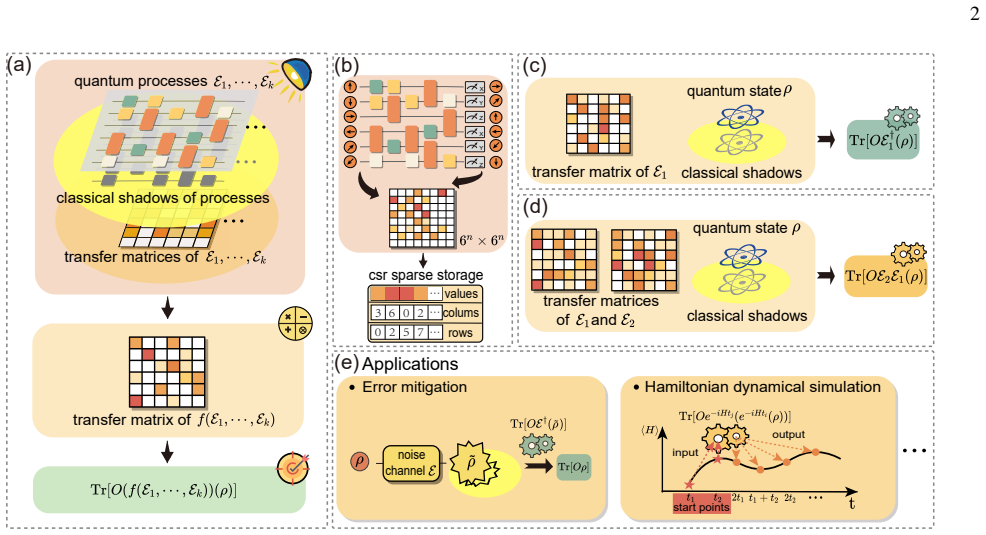
Shadow engineering encodes the classical shadows of processes into sparse transfer matrices to predict f(E1, E2, ..., Ek) properties with proven polynomial sample complexity, matching single-channel efficiency while exponentially lower than quantum process tomography, without physical execution of the composite process.
What carries the argument
Sparse transfer matrices that algebraically combine individual process shadows to reproduce composite statistics.
Load-bearing premise
Individual process shadows can be encoded into sparse transfer matrices whose algebraic combinations accurately reproduce the statistics of the composite process without extra assumptions on the form of the function or the noise model.
What would settle it
An experiment in which the statistics predicted by combining the sparse transfer matrices differ measurably from direct measurements of the composite process on the same hardware.
Figures
read the original abstract
Characterizing quantum processes is essential for hardware benchmarking, error diagnosis, and algorithm verification. While recent work [PRX QUANTUM \textbf{4}, 040337 (2023)] extended classical shadows from quantum state to quantum process, enabling efficient single-channel $\mathcal{E}$ property prediction, its applicability to composite processes $f(\mathcal{E}_1, \mathcal{E}_2,\cdots, \mathcal{E}_k)$ remains unexplored. We introduce shadow engineering, a framework encoding the classical shadows of processes into sparse transfer matrices to predict $f(\mathcal{E}_1, \mathcal{E}_2,\cdots, \mathcal{E}_k)$ properties with proven polynomial sample complexity, matching single-channel efficiency while exponentially lower than quantum process tomography. Crucially, this approach repurposes existing $\mathcal{E}_m$-shadow data without physical execution of $f(\mathcal{E}_1, \mathcal{E}_2,\cdots, \mathcal{E}_k)$, enabling flexible quantum process characterization with minimal hardware overhead. We demonstrate the framework's effectiveness and practicality on a superconducting quantum processor for typical applications such as error mitigation and Hamiltonian dynamical simulation. This framework unlocks new capabilities for predicting complex quantum behaviors without physical re-execution, with immediate applications in near-term device calibration and quantum simulation.
Editorial analysis
A structured set of objections, weighed in public.
Referee Report
Summary. The manuscript introduces shadow engineering, a framework that encodes classical shadows of individual quantum processes into sparse transfer matrices. This enables prediction of properties of composite functions f(ℰ₁, ℰ₂, …, ℰₖ) with claimed polynomial sample complexity, matching single-channel shadow efficiency while avoiding physical execution of the composite process and exponentially improving on quantum process tomography. The approach is demonstrated on a superconducting processor for error mitigation and Hamiltonian dynamical simulation.
Significance. If the encoding and algebraic combination steps are shown to hold for general f without hidden restrictions, the result would enable flexible, low-overhead characterization of composite quantum processes by repurposing existing shadow data, with clear practical value for near-term device calibration and simulation.
major comments (1)
- [Abstract / framework introduction] Abstract and framework section: the central claim that sparse transfer-matrix combinations of individual ℰₘ shadows exactly reproduce measurement statistics for arbitrary (including nonlinear) f without extra assumptions on f or the noise model is load-bearing. For f involving products of distinct expectation values, e.g., Tr[O₁ ℰ₁(ρ)]·Tr[O₂ ℰ₂(ρ)], it is unclear how addition or multiplication of the matrices captures the required cross terms; an explicit derivation or counter-example check is needed.
minor comments (2)
- Specify the precise algebraic operations (addition, multiplication, Kronecker, etc.) used for different classes of f and confirm they remain polynomial in the number of processes.
- Clarify data-exclusion rules and error-bound derivations referenced in the abstract's polynomial-complexity statement.
Simulated Author's Rebuttal
We thank the referee for their careful reading of the manuscript and for identifying this key point about the generality of the framework. We address the concern directly below and have revised the manuscript to include the requested explicit derivation and verification.
read point-by-point responses
-
Referee: [Abstract / framework introduction] Abstract and framework section: the central claim that sparse transfer-matrix combinations of individual ℰₘ shadows exactly reproduce measurement statistics for arbitrary (including nonlinear) f without extra assumptions on f or the noise model is load-bearing. For f involving products of distinct expectation values, e.g., Tr[O₁ ℰ₁(ρ)]·Tr[O₂ ℰ₂(ρ)], it is unclear how addition or multiplication of the matrices captures the required cross terms; an explicit derivation or counter-example check is needed.
Authors: The sparse transfer matrices encode each process shadow such that linear compositions (concatenation, parallel application) are realized exactly by matrix addition and multiplication, reproducing the composite measurement statistics in expectation. For nonlinear f, including products of distinct expectation values such as Tr[O₁ ℰ₁(ρ)] · Tr[O₂ ℰ₂(ρ)], the nonlinearity is applied after the individual scalar estimates are obtained from their respective shadows; the product is formed from the two independent estimators. Because the shadows are collected in separate experiments, no cross terms arise inside the matrix algebra itself. The expectation of the product estimator remains unbiased, and the sample complexity stays polynomial because the variance of the product is controlled by the individual shadow variances (via standard concentration bounds). We have added an explicit derivation of this construction for general f (including the product example) together with a numerical counter-example verification in the revised manuscript (new subsection 3.2 and Appendix C). No additional assumptions on f or the noise model are required beyond those of the underlying single-channel shadow protocol. revision: yes
Circularity Check
No circularity; derivation self-contained via independent shadow data repurposing
full rationale
The abstract and framework description introduce shadow engineering as an encoding of existing process shadows into sparse transfer matrices for composite prediction, without any quoted reduction of the claimed polynomial-complexity predictions to quantities fitted from the target data itself. The cited prior work on single-channel shadows is treated as external input, and no self-citation chain or definitional loop is exhibited that would force the composite f predictions by construction. The method is presented as repurposing independent data, consistent with a non-circular extension of classical shadows.
Axiom & Free-Parameter Ledger
axioms (1)
- domain assumption Quantum processes admit a linear transfer-matrix representation that can be sparsely encoded from classical shadows.
Reference graph
Works this paper leans on
-
[1]
Mohseni, A
M. Mohseni, A. T. Rezakhani, and D. A. Lidar, Phys. Rev. A 77, 032322 (2008)
2008
-
[2]
J. L. O’Brien, G. J. Pryde, A. Gilchrist, D. F. V . James, N. K. Langford, T. C. Ralph, and A. G. White, Phys. Rev. Lett.93, 080502 (2004)
2004
-
[3]
A. J. Scott, J. Phys. A: Math. Theor.41, 055308 (2008)
2008
-
[4]
Sugiyama, S
T. Sugiyama, S. Imori, and F. Tanaka, Phys. Rev. A103, 062615 (2021)
2021
-
[5]
Torlai, C
G. Torlai, C. J. Wood, A. Acharya, G. Carleo, J. Carrasquilla, and L. Aolita, Nat. Commun.14, 2858 (2023)
2023
-
[6]
J. B. Altepeter, D. Branning, E. Jeffrey, T. C. Wei, P. G. Kwiat, R. T. Thew, J. L. O’Brien, M. A. Nielsen, and A. G. White, Phys. Rev. Lett.90, 193601 (2003)
2003
-
[7]
Huang, R
H.-Y . Huang, R. Kueng, and J. Preskill, Nat. Phys.16, 1050 (2020)
2020
-
[8]
Zhang, J
T. Zhang, J. Sun, X.-X. Fang, X.-M. Zhang, X. Yuan, and H. Lu, Phys. Rev. Lett.127, 200501 (2021)
2021
-
[9]
S. Chen, W. Yu, P. Zeng, and S. T. Flammia, PRX Quantum2, 030348 (2021)
2021
-
[10]
Struchalin, Y
G. Struchalin, Y . A. Zagorovskii, E. Kovlakov, S. Straupe, and S. Kulik, PRX Quantum2, 010307 (2021)
2021
-
[11]
Huang, Nat
H.-Y . Huang, Nat. Rev. Phys.4, 81 (2022)
2022
-
[12]
Elben, S
A. Elben, S. T. Flammia, H.-Y . Huang, R. Kueng, J. Preskill, B. Vermersch, and P. Zoller, Nat. Rev. Phys.5, 9 (2023)
2023
-
[13]
Acharya, S
A. Acharya, S. Saha, and A. M. Sengupta, Phys. Rev. A104, 052418 (2021)
2021
-
[14]
A. A. Akhtar, H.-Y . Hu, and Y .-Z. You, Quantum7, 1026 (2023)
2023
-
[15]
D. E. Koh and S. Grewal, Quantum6, 776 (2022)
2022
-
[16]
Jnane, J
H. Jnane, J. Steinberg, Z. Cai, H. C. Nguyen, and B. Koczor, PRX Quantum5, 010324 (2024). 6
2024
-
[17]
Ippoliti, Y
M. Ippoliti, Y . Li, T. Rakovszky, and V . Khemani, Phys. Rev. Lett.130, 230403 (2023)
2023
-
[18]
Zhou and Q
Y . Zhou and Q. Liu, Quantum7, 1044 (2023)
2023
-
[19]
H.-Y . Hu, A. Gu, S. Majumder, H. Ren, Y . Zhang, D. S. Wang, Y .-Z. You, Z. Minev, S. F. Yelin, and A. Seif, Nat. Commun.16, 2943 (2025)
2025
-
[20]
Jamiołkowski, Rep
A. Jamiołkowski, Rep. Math. Phys.3, 275 (1972)
1972
-
[21]
D. W. Leung, J. Math. Phys.44, 528 (2003)
2003
-
[22]
Kunjummen, M
J. Kunjummen, M. C. Tran, D. Carney, and J. M. Taylor, Phys. Rev. A107, 042403 (2023)
2023
-
[23]
R. Levy, D. Luo, and B. K. Clark, Phys. Rev. Res.6, 013029 (2024)
2024
-
[24]
Wang and K
H. Wang and K. He, Phys. Rev. A112, 012413 (2025)
2025
-
[25]
Huang, S
H.-Y . Huang, S. Chen, and J. Preskill, PRX Quantum4, 040337 (2023)
2023
- [26]
-
[27]
Huang, X.-Y
H.-L. Huang, X.-Y . Xu, C. Guo, G. Tian, S.-J. Wei, X. Sun, W.- S. Bao, and G.-L. Long, Sci. China-Phys. Mech. Astron.66, 250302 (2023)
2023
-
[28]
Suzuki, S
Y . Suzuki, S. Endo, K. Fujii, and Y . Tokunaga, PRX Quantum 3, 010345 (2022)
2022
-
[29]
Z. Cai, R. Babbush, S. C. Benjamin, S. Endo, W. J. Huggins, Y . Li, J. R. McClean, and T. E. O’Brien, Rev. Mod. Phys.95, 045005 (2023)
2023
-
[30]
J. Haah, M. B. Hastings, R. Kothari, and G. H. Low, SIAM J. Comput.52, FOCS18 (2021)
2021
-
[31]
Q. Zhao, Y . Zhou, A. F. Shaw, T. Li, and A. M. Childs, Phys. Rev. Lett.129, 270502 (2022)
2022
-
[32]
G. H. Golub and C. F. Van Loan,Matrix Computations, 4th ed. (Johns Hopkins University Press, Philadelphia, PA, 2013)
2013
-
[33]
J. Gao, W. Ji, F. Chang, S. Han, B. Wei, Z. Liu, and Y . Wang, ACM Comput. Surv.55, 244 (2023)
2023
- [34]
-
[35]
Rossini, D
M. Rossini, D. Maile, J. Ankerhold, and B. I. C. Donvil, Phys. Rev. Lett.131, 110603 (2023)
2023
-
[36]
Zhang, P.-Y
W.-M. Zhang, P.-Y . Lo, H.-N. Xiong, M. W.-Y . Tu, and F. Nori, Phys. Rev. Lett.109, 170402 (2012)
2012
-
[37]
P. Zeng, J. Sun, L. Jiang, and Q. Zhao, PRX Quantum6, 010359 (2025)
2025
-
[38]
Chakraborty, Quantum8, 1496 (2024)
S. Chakraborty, Quantum8, 1496 (2024)
2024
-
[39]
Shadow Engineering of Quantum Processes
I. Loaiza, A. Sankar Brahmachari, and A. F. Izmaylov, Quan- tum Sci. Technol.10, 035035 (2025). Supplemental Material for “Shadow Engineering of Quantum Processes” SHADOW ENGINEERING FRAMEWORK Given an observableO, an input stateρ, and classical shadows ofkunknown quantum processes{E m}k m=1, the target of shadow engineering is to predict the expected val...
2025
-
[40]
For each case, we elaborate on the construction of the corresponding transfer matrix and analyze the scaling behavior of the prediction error
and process concatenation (E 2 ◦ E 1). For each case, we elaborate on the construction of the corresponding transfer matrix and analyze the scaling behavior of the prediction error. Shadow engineering for predicting T r[OE † 1(ρ)] We first consider the casef(E 1) =E †
-
[41]
1, the transfer matrices ofE 1 andE † 1 satisfy TE † 1 =T † E1
By Lem. 1, the transfer matrices ofE 1 andE † 1 satisfy TE † 1 =T † E1 . While Lem. 1 establishes the adjoint relation for ideal transfer matrices, we cannot directly estimateT E † 1 by taking the adjoint of the empirical estimate ˆT † E1–this is because ˆT † E1 may fail to satisfy the property that the sum of each row equals 1. Under the uniform input di...
-
[42]
,T1[5]}(S76) whereT 1[i] denotes thei-th row vector ofT 1
DefineT ini as the set of 6 row vectors ofT 1: Tini ={T 1[0],T 1[1], . . . ,T1[5]}(S76) whereT 1[i] denotes thei-th row vector ofT 1. 13
-
[43]
Compute then-fold tensor product ofT ini: Tn =T ⊗n ini (S77)
-
[44]
O 6n X b=1 ( ˆTE1)cb 6n X a=1 (Tn)ba 6n X l=1 ( ˆTE2)alM−1(S ⊗n l ) # −Tr
Assemble the resulting 6 n ×6 n matrix by treating each element ofT n as a row vector. Then-qubit matrixT n inherits exponential sparsity fromT 1. StoringT n in CSR format dramatically reduces both memory requirements and computational complexity. Using the classical shadowsS N1(E1) andS N2(E2), we computed the estimated transfer matrix ˆTE2◦E1. Within th...
-
[45]
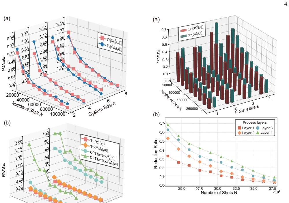
Across all tested system sizes, QPT exhibits significantly larger errors than shadow engineering across all system sizes
-
[46]
QPT’s predictions for the composite observable Tr[OE 2E1(ρ)] suffer from severe error propagation due to inde- pendent tomography of each channel
-
[47]
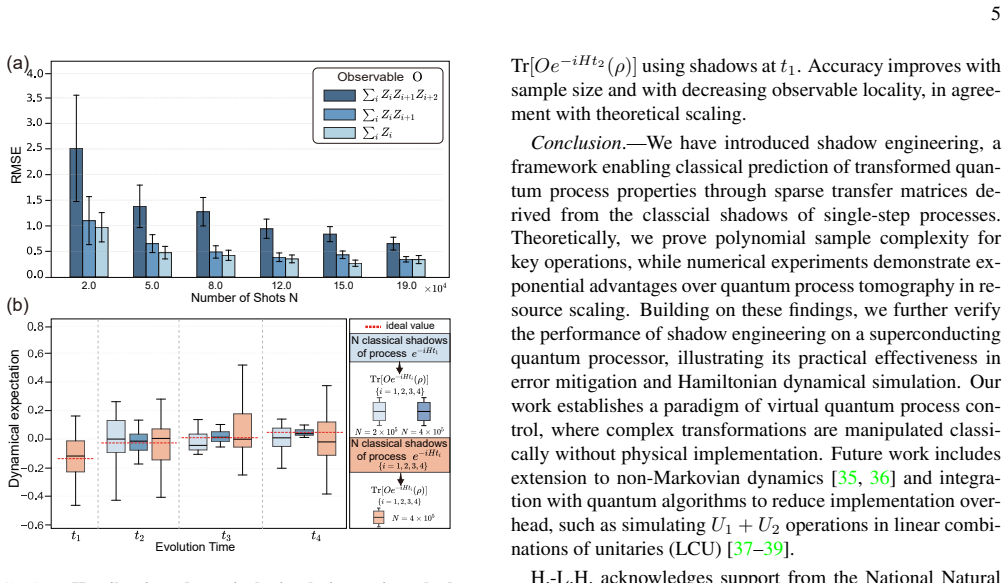
NY i=1 RXi(2ht) # ·
The performance gap between shadow engineering and QPT widens as qubit count increases. This fundamental performance gap originates from their inherent sample complexity scalings: shadow engineering achieves polynomial scaling in both measurement resources and computational cost, whereas standard QPT inevitably incurs exponential overhead with increasing ...
2020
discussion (0)
Sign in with ORCID, Apple, or X to comment. Anyone can read and Pith papers without signing in.