REVIEW 4 major objections 6 minor 58 references
Rethinking Timing Residuals: Advancing PET Detectors with Explicit TOF Corrections
T0 review · 4 major / 6 minor · reviewed 2026-08-08 · deepseek-v4-flash
Pith's one-line read The paper redefines the timing residual as half the measured-minus-expected time difference, enabling explicit per-event TOF corrections that improve CTR from (371±6) ps to (281±5) ps with a single source position.
desk verdict Explicit residual TOF correction genuinely improves on implicit models and enables single-position training; the 281 ps headline, however, comes from a 33×33 in-plane grid, not a true point source. read the letter →
The pith
A machine-rendered reading of the paper's core claim, the machinery that carries it, and where it could break.
The reading
What carries the argument
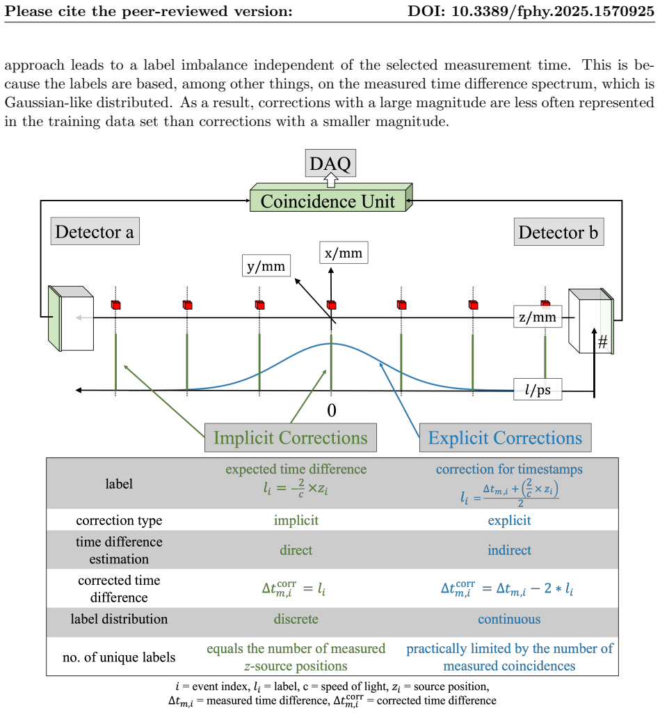
The central object is the redefined timing residual label $r_i = (\Delta t_{m,i} - \Delta t_E(z_i))/2 = (\Delta t_{m,i} + 2 z_i / c)/2$, used as the regression target for gradient-boosted decision trees. It carries the argument by converting the calibration problem from predicting an absolute expected time difference (implicit) to predicting a per-event skew correction (explicit), which makes the label distribution independent of source-position sampling and lets a model trained at $z = 0$ provide corrections for all $z$. The rest of the machinery is the two-stage residual physics scheme: a first-order analytical timestamp skew calibration removes position-independent offsets, and the ML model is trained only on the remaining higher-order, event-dependent deviations, with the appendix's linearity argument assuming that predictions equal labels.
What would settle it
Move a point source to several $z$-positions, train an explicit model using only the $z=0$ data, and compare its predicted corrections with those of a model trained on all positions: if the per-event residual $\delta_i = (\Delta t_{m,i} + 2 z_i / c)/2$ shifts with $z$ by more than the detector's timing resolution, the single-position assumption fails.
Extended reading notes
Core claim
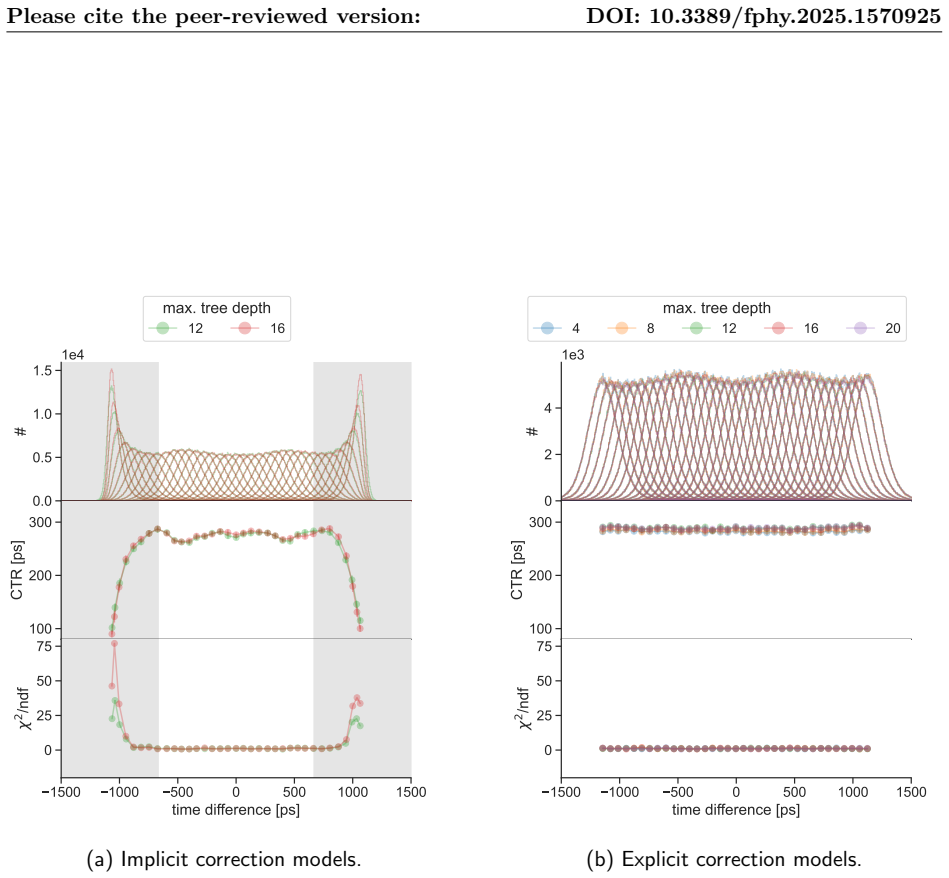
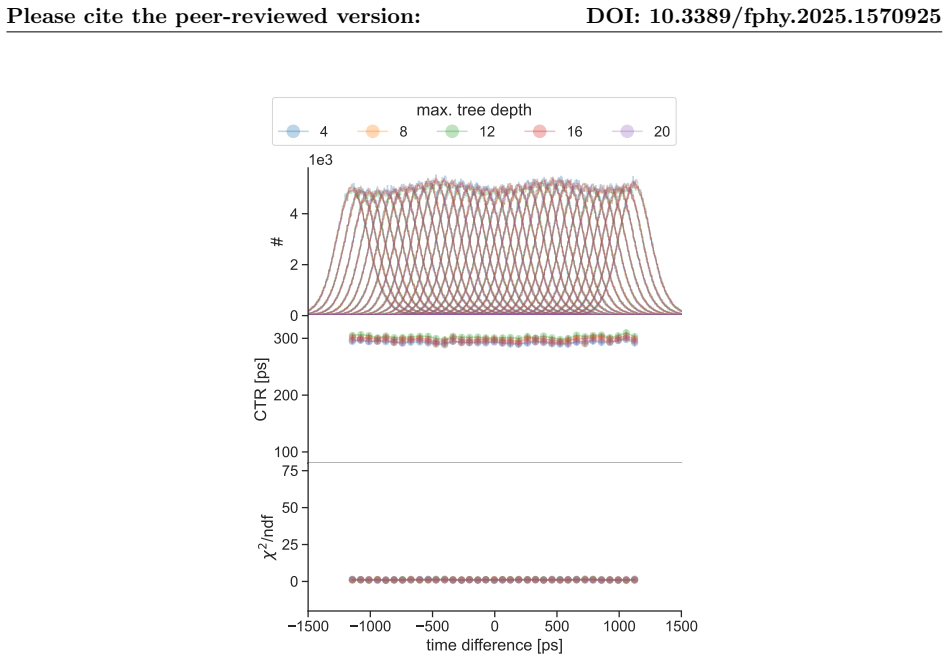
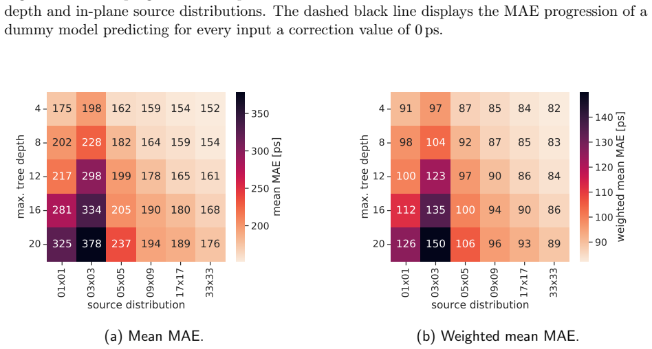
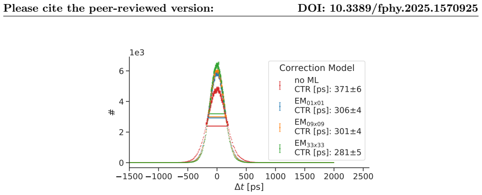
The paper's central claim is that the residual physics-based calibration concept reaches its full practical value when the timing residual is defined as $r_i = (\Delta t_{m,i} - \Delta t_E(z_i))/2$, because then a model's output is itself the timestamp correction ($t_{a,i} \leftarrow t_{a,i} - r_i$, $t_{b,i} \leftarrow t_{b,i} + r_i$) instead of a predicted corrected time difference. This restores a translational symmetry to the labeling: shifting the source shifts the expected time difference and the measured time difference by the same amount, so the label distribution no longer encodes source position. The authors demonstrate that explicit-correction gradient-boosted trees are immune to the step-width collapse observed for implicit models, remain linear across the full $\pm170$ mm test range, and improve timing resolution from $(371 \pm 6)$ ps to $(281 \pm 5)$ ps for 430–590 keV coincidences; a model trained on a single centered point source still reaches $(306 \pm 4)$ ps, and a $33 \times 33$ in-plane distribution reaches $(281 \pm 5)$ ps. They interpret the small degradation relative to the best implicit model as acceptable given the simplification in acquisition and the exponential reduction in model size (tree depth 4 instead of 18).
Load-bearing premise
The method assumes that, after the first analytical time-skew calibration, whatever timing error remains in an event does not depend on where the radiation source sits between the detectors, so a model trained with the source at one position works for all positions.
Editorial extensions
If this is right
- Explicit-correction models trained with coarse axial sampling (50 mm or 100 mm step width) generalize to unseen 10 mm-sampled positions, whereas implicit models oscillate and fail linearity checks.
- A single centered source position is enough to train an explicit model, removing the requirement for a motorized multi-position translation stage in calibration.
- The explicit formulation preserves linearity over the full $\pm170$ mm test range, so TOF information remains interpretable for image reconstruction.
- Because shallow trees (depth 4) suffice, model memory shrinks by a factor of about $2^{18-4}$, making the correction suitable for FPGA-based, high-throughput PET readout.
- Both correction approaches correct time-walk effects well: enlarging the energy window from 430–590 keV to 300–700 keV degrades CTR only slightly (about 2\%) for explicit models, versus about 20\% without ML.
Reading between the lines
- Editorial inference: the independence of the explicit label from source position is a symmetry argument, not a proof that all per-event skews are position-independent; the transferability of a $z=0$-trained model to off-center positions should be re-tested for detectors with stronger depth-of-interaction-dependent skews.
- Editorial inference: the comparison between 1×1 and 33×33 in-plane distributions is confounded by a $33^2$ difference in training statistics, so the observation that 3×3 performs worse than 1×1 is the cleanest evidence that source arrangement itself matters; a matched-statistics experiment would separate the two effects.
- Editorial inference: because the explicit residual is defined from the measured time difference and the geometric expected time difference, the same label construction could be applied to any coincidence pair with a known geometric time-difference model, such as dual-sided readout or monolithic detectors, provided the single-position assumption holds.
- Editorial inference: a testable extension is to train explicitly on data from one detector stack and apply it to an unseen stack of the same design; the paper lists this as future work and expects feature-based robustness.
Editorial analysis
A structured set of objections, weighed in public.
Referee Report
Summary. The paper proposes an explicit timing-residual formulation for machine-learning-based TOF calibration in PET detectors. The label is defined as half of the difference between the measured time difference and the expected time difference from the known source position, r_i = (Δt_m,i − Δt_E(z_i))/2, which yields a continuous label distribution that is claimed to be independent of the number of source positions along the transaxial axis. The authors compare this explicit-correction approach with their earlier implicit-correction models using a three-stage evaluation (MAE, linearity/ε, and CTR) on real data from two 4×4 LYSO:Ce,Ca detector blocks coupled to Broadcom NUV-MT SiPMs and read out with TOFPET2. They report an improvement in CTR from (371±6) ps to (281±5) ps for 430–590 keV coincidences, robustness to spatial undersampling, preserved linearity over the full test range, and a large reduction in model size suitable for FPGA deployment.
Significance. If the results hold, the explicit residual formulation is a practically valuable contribution: it removes the need for dense transaxial source sampling, preserves linearity over the full test range, and yields compact tree ensembles suitable for high-throughput PET applications. The three-stage evaluation is thorough, uncertainties are reported, and the comparison with implicit models is informative. The main weaknesses are that the central transfer claim—that a model trained at a single z-plane corrects events at all z—rests on an assumption about the z-independence of residual skews that is not proven, and the headline CTR is obtained with a 33×33 in-plane grid rather than the single-point-source configuration emphasized in the abstract.
major comments (4)
- [Appendix, Eq. (25)] The linearity argument assumes predictions equal labels (p_i ≈ l_i) and then derives E[Δt_corr] = E[Δt]. This is circular because the property to be established is precisely that the model's predictions, which cannot depend on z since z is not a feature, equal the label l_i = (Δt_m,i − Δt_E(z_i))/2 for all z_i. For a model trained only at z=0, l_i reduces to Δt_m,i/2, and no argument in the appendix shows that this equality survives at z≠0. Please provide a non-circular derivation or a direct empirical demonstration that the residual skew δ_i is independent of z after the first-order calibration.
- [Abstract and Table 3] The headline improvement to (281±5) ps is obtained by model EM33x33, which uses 33×33 = 1089 in-plane source positions; the single-point-source model EM01x01 reaches (306±4) ps (Table 3). Since the paper's key simplifying claim is that acquisition reduces to a single source position, presenting the 281 ps value as the headline conflates the best-possible calibration with the single-source calibration. The abstract and Section 4 should either report the single-source value as the headline for the simplification claim or explicitly separate the two achievements.
- [Section 2.6.2 and Section 5] The single-position transfer result rests on the assumption that, after the analytical first-order time-skew calibration, the per-event residual skew δ_i is independent of z (DOI and incidence-angle effects in 20-mm crystals could violate this). The current evidence is limited to one detector pair, and the paper itself defers cross-stack stability to future work. To support the central claim, please add a quantitative analysis of CTR as a function of |z| for a model trained only at z=0, including the range over which the single-source model stays within a pre-specified tolerance of the full multi-position model.
- [Section 3.1.3 and Tables 1–3] Hyperparameters (tree depth) are selected from a grid evaluated on the same test data used to report CTR. The CTR differences among depths are small (e.g., 281±5 vs 287±5 ps), so selection-on-test can bias the reported improvement. Use a separate validation set for hyperparameter selection, or report the full distribution of CTR across depths and a correction for multiple comparisons.
minor comments (6)
- [Section 2.3] The sentence "we propose to redefine the residuals" should refer to redefining the labels; also "high coverade" is misspelled (should be "high coverage").
- [Figure 3 caption] The caption would benefit from a verb: "the implicit model IM10,12 and the explicit model EM10,4 are used" reads more clearly.
- [Section 2.4.2, Eq. (11)] The notation would benefit from an explicit statement that µ is the fitted mean of the prediction distribution and that ε is the parameter being estimated.
- [Section 4] The phrase "capable of proving good results" should be "capable of providing good results" or "showing good results".
- [Appendix, Eq. (26)] The expectation expression contains unmatched brackets and non-standard delimiters from the LaTeX source; please correct the typesetting.
- [Tables 1, 3, 5, 6] The placement of the CTR tables could be improved: Table 3 (the main in-plane result) appears before the extended energy-window tables, but the text in Section 3.2.3 refers to them in a way that is hard to follow; consider renumbering or adding in-text pointers.
Circularity Check
The appendix's linearity argument is tautological (predictions assumed to equal labels), and the single-source z-transfer claim presupposes a z-independent residual skew; the headline CTR improvement is nevertheless an independent measured result.
-
self definitional
[Appendix, 'Consideration of the Linearity of Explicit Correction Models', Eqs. (24)-(28)]
"If we assume that the explicit correction model was successfully trained, we can approximate the predictions by the labels (see Eq. (6)), pi ≈ li := Δtm,i − ΔtE(z)/2. Inserting Eq. (25) into Eq. (24), yields ΔtE = E[{Δti − 2 · (Δti − E[{Δti}])/2}] = E[{E[{Δti}]}] = E[{Δti}], which is the expected time difference for the non-corrected timestamps."
The linearity 'result' is obtained by substituting the label definition for the model prediction and simplifying; it assumes exactly what the model is supposed to provide (pi = li). The corrected mean then equals the uncorrected mean by construction, independent of any learned model property. The paper itself states 'we will not provide a formal proof' and calls it 'basic understanding', but Section 4 cites this appendix as the mathematical reasoning for the claimed source-location robustness ('The robustness of the explicit correction models is reasoned by the way the residuals are defined'). The empirical χ2/ε and CTR evaluations are independent evidence, so this is a partial, not total, circularity.
full rationale
The central empirical claims are independently measured: the CTR improvements in Tables 1-4 are obtained on held-out test data against a 'no ML' analytical baseline, and the linearity/ε evaluations in Section 3.1.2 and 3.2.2 use real source-position scans. No load-bearing self-citation chain was found: prior works [44-46,51] are used for comparison and for the implicit-correction baseline, not as the justification for the explicit-correction result. The genuine circular step is confined to the appendix, where the linearity robustness is 'derived' by assuming predictions equal labels; this reduces to the label construction and is not a model property. The z-independence/single-position transfer is an empirical assumption about post-calibration skew being independent of source position, validated here for one detector pair and explicitly deferred for cross-stack stability in the Outlook; it is not circular, but it is the load-bearing assumption behind the 'single source position' simplification. Note also that the headline 281 ± 5 ps comes from EM33x33 (1089 in-plane positions), while the true single-point model EM01x01 reaches 306 ± 4 ps, weakening the 'single source position' framing without making it circular. Overall, the only reduction-by-construction is the appendix's consistency check, so the score is moderate rather than severe.
Assumptions & free parameters
free parameters (8)
- XGBoost learning rate =
0.1
- Maximum number of trees =
1000
- Maximum tree depth =
d in {4,8,12,16,20}; best CTR 281 ps at d=4
- Number of relative timestamps per detector =
na=12, nb=9
- Energy exclusion thresholds for hits =
2.5 and 100 arbitrary units
- Cluster and coincidence windows =
8 ns cluster, 50 ns software coincidence
- Evaluation energy window =
430-590 keV primary; 300-700 keV secondary
- First-order time skew calibration offsets =
not reported
assumptions (6)
- domain assumption Timestamp decomposition td = Θ + Δts (Eq. 1)
- domain assumption After first-order analytical calibration, remaining skews are event-dependent higher-order effects that ML can learn
- domain assumption The residual timing skew is independent of source position z (translation invariance)
- domain assumption Supervised labels from a 22Na source position give unbiased expected time differences via ΔtE = -2z/c (Eq. 3)
- domain assumption Input features (SiPM timestamps, energies, IDs, light moments) contain sufficient information to predict the residual
- ad hoc to paper The appendix linearity argument assumes predictions equal labels (p_i ≈ l_i)
Cite this review
Pith. "Pith review of Rethinking Timing Residuals: Advancing PET Detectors with Explicit TOF Corrections." pith.science (2026). https://pith.science/paper/MAKPU3QX
@misc{pith2026250207630,
  author       = {Pith},
  title        = {Pith review of: Rethinking Timing Residuals: Advancing PET Detectors with Explicit TOF Corrections},
  year         = {2026},
  howpublished = {\url{https://pith.science/paper/MAKPU3QX}},
  note         = {Machine review of arXiv:2502.07630}
}
abstract
PET is a functional imaging method that visualizes metabolic processes. TOF information can be derived from coincident detector signals and incorporated into image reconstruction to enhance the SNR. PET detectors are typically assessed by their CTR, but timing performance is degraded by various factors. Research on timing calibration seeks to mitigate these degradations and restore accurate timing information. While many calibration methods use analytical approaches, machine learning techniques have recently gained attention due to their flexibility. We developed a residual physics-based calibration approach that combines prior domain knowledge with the power of machine learning models. This approach begins with an initial analytical calibration addressing first-order skews. The remaining deviations, regarded as residual effects, are used to train machine learning models to eliminate higher-order skews. The key advantage is that the experimenter guides the learning process through the definition of timing residuals. In earlier studies, we developed models that directly predicted the expected time difference, which offered corrections only implicitly (implicit correction models). In this study, we introduce a new definition for timing residuals, enabling us to train models that directly predict correction values (explicit correction models). The explicit correction approach significantly simplifies data acquisition, improves linearity, and enhances timing performance from $371 \pm 6$ ps to $281 \pm 5$ ps for coincidences from 430 keV to 590 keV. Additionally, the new definition reduces model size, making it suitable for high-throughput applications like PET scanners. Experiments were conducted using two detector stacks composed of $4 \times 4$ LYSO:Ce,Ca crystals ($3.8\times 3.8\times 20$ mm$^{3}$) coupled to $4 \times 4$ Broadcom NUV-MT SiPMs and digitized with the TOFPET2 ASIC.
Figures


Figures from the paper (14 more)






Reference graph
Works this paper leans on
-
[1]
Benefit of Time-of-Flight in PET: Experimental and Clinical Results
Joel S. Karp et al. “Benefit of Time-of-Flight in PET: Experimental and Clinical Results.” In: Journal of Nuclear Medicine49.3 (Mar. 2008). Publisher: Society of Nuclear Medicine Section: BASIC SCIENCE INVESTIGATIONS, pp. 462–470. doi: 10.2967/jnumed.107.044834
-
[2]
Impact of Time-of-Flight on PET Tumor Detection
Dan J. Kadrmas et al. “Impact of Time-of-Flight on PET Tumor Detection.” In: Journal of Nuclear Medicine 50.8 (Aug. 2009). Publisher: Society of Nuclear Medicine Section: BASIC SCIENCE INVESTIGATIONS, pp. 1315–1323. doi: 10.2967/jnumed.109.063016
-
[3]
Roadmap toward the 10 ps time-of-flight PET challenge
Paul Lecoq et al. “Roadmap toward the 10 ps time-of-flight PET challenge.” In: Physics in Medicine & Biology65.21 (Oct. 2020). Publisher: IOP Publishing, 21RM01. doi: 10.1088/ 1361-6560/ab9500
work page 2020
-
[4]
Mythra Varun Nemallapudi et al. “Sub-100 ps coincidence time resolution for positron emis- sion tomography with LSO:Ce codoped with Ca.” In: Physics in Medicine & Biology60.12 (May 2015). Publisher: IOP Publishing, p. 4635. doi: 10.1088/0031-9155/60/12/4635
-
[5]
Vanessa Nadig et al. “Timing advances of commercial divalent-ion co-doped LYSO:Ce and SiPMs in sub-100 ps time-of-flight positron emission tomography.” In: Physics in Medicine & Biology 68.7 (Mar. 2023). Publisher: IOP Publishing, p. 075002. doi: 10 . 1088 / 1361 - 6560/acbde4
work page 2023
-
[6]
Studies on the Cherenkov Effect for Improved Time Resolution of TOF- PET
S. E. Brunner et al. “Studies on the Cherenkov Effect for Improved Time Resolution of TOF- PET.” In: IEEE Transactions on Nuclear Science61.1 (Feb. 2014). Conference Name: IEEE Transactions on Nuclear Science, pp. 443–447. doi: 10.1109/TNS.2013.2281667
arXiv 2014
-
[7]
Time Resolution Studies of Thallium Based Cherenkov Semiconduc- tors
Giulia Terragni et al. “Time Resolution Studies of Thallium Based Cherenkov Semiconduc- tors.” In: Frontiers in Physics 10 (Mar. 2022). Publisher: Frontiers. doi: 10.3389/fphy. 2022.785627
arXiv 2022
-
[8]
BGO as a hybrid scintillator / Cherenkov radiator for cost- effective time-of-flight PET
S. E. Brunner and D. R. Schaart. “BGO as a hybrid scintillator / Cherenkov radiator for cost- effective time-of-flight PET.” In: Physics in Medicine & Biology62.11 (May 2017). Publisher: IOP Publishing, p. 4421. doi: 10.1088/1361-6560/aa6a49
Show all 58 references
-
[9]
Exploring Cherenkov Emis- sion of BGO for TOF-PET
Nicolaus Kratochwil, Etiennette Auffray, and Stefan Gundacker. “Exploring Cherenkov Emis- sion of BGO for TOF-PET.” In: IEEE Transactions on Radiation and Plasma Medical Sci- ences 5.5 (Sept. 2021). Conference Name: IEEE Transactions on Radiation and Plasma Med- ical Sciences,...
2021
-
[10]
Cherenkov Radiation–Based Coincidence Time Resolution Measurements in BGO Scintillators
Andrea Gonzalez-Montoro et al. “Cherenkov Radiation–Based Coincidence Time Resolution Measurements in BGO Scintillators.” In: Frontiers in Physics 10 (Jan. 2022). Publisher: Frontiers. doi: 10.3389/fphy.2022.816384
2022
-
[11]
Scintillation and cherenkov pho- ton counting detectors with analog silicon photomultipliers for TOF-PET
Joshua W. Cates, Woon-Seng Choong, and Erik Brubaker. “Scintillation and cherenkov pho- ton counting detectors with analog silicon photomultipliers for TOF-PET.” In: Physics in Medicine & Biology69.4 (Feb. 2024). Publisher: IOP Publishing, p. 045025. doi: 10.1088/ 1361-6560/ad2125
2024
-
[13]
Metascintillators for Ultrafast Gamma Detectors: A Review of Current State and Future Perspectives
Georgios Konstantinou et al. “Metascintillators for Ultrafast Gamma Detectors: A Review of Current State and Future Perspectives.” In: IEEE Transactions on Radiation and Plasma Medical Sciences 6.1 (Jan. 2022). Conference Name: IEEE Transactions on Radiation and Plasma Medical...
2022
-
[14]
A proof-of-concept of cross-luminescent metascintillators: testing results on a BGO:BaF2 metapixel
G. Konstantinou et al. “A proof-of-concept of cross-luminescent metascintillators: testing results on a BGO:BaF2 metapixel.” In: Physics in Medicine & Biology 68.2 (Jan. 2023). Publisher: IOP Publishing, p. 025018. doi: 10.1088/1361-6560/acac5f
2023 doi
-
[15]
Improving the Time Resolution of TOF-PET Detectors by Double-Sided Readout
Stefan Seifert and Dennis R. Schaart. “Improving the Time Resolution of TOF-PET Detectors by Double-Sided Readout.” In: IEEE Transactions on Nuclear Science 62.1 (Feb. 2015). Conference Name: IEEE Transactions on Nuclear Science, pp. 3–11. doi: 10 . 1109 / TNS . 2014.2368932
2015
-
[16]
A 32 mm × 32 mm × 22 mm monolithic LYSO:Ce detector with dual-sided digital photon counter readout for ultrahigh-performance TOF-PET and TOF- PET/MRI
Giacomo Borghi et al. “A 32 mm × 32 mm × 22 mm monolithic LYSO:Ce detector with dual-sided digital photon counter readout for ultrahigh-performance TOF-PET and TOF- PET/MRI.” In: Physics in Medicine & Biology61.13 (June 2016). Publisher: IOP Publishing, p. 4929. doi: 10.1088/0...
2016 doi
-
[17]
Improved image quality using monolithic scintillator detectors with dual-sided readout in a whole-body TOF-PET ring: a simulation study
Valerio Tabacchini et al. “Improved image quality using monolithic scintillator detectors with dual-sided readout in a whole-body TOF-PET ring: a simulation study.” In: Physics in Medicine & Biology62.5 (Feb. 2017). Publisher: IOP Publishing, p. 2018. doi: 10.1088/ 1361-6560/aa56e1
2017
-
[19]
High-frequency SiPM readout advances measured coincidence time resolution limits in TOF-PET
Stefan Gundacker et al. “High-frequency SiPM readout advances measured coincidence time resolution limits in TOF-PET.” In:Physics in Medicine & Biology64.5 (Feb. 2019), p. 055012. doi: 10.1088/1361-6560/aafd52
2019 doi
-
[20]
Low power implementation of high frequency SiPM readout for Cherenkov and scintillation detectors in TOF-PET
Joshua W Cates and Woon-Seng Choong. “Low power implementation of high frequency SiPM readout for Cherenkov and scintillation detectors in TOF-PET.” In:Physics in Medicine & Biology 67.19 (Oct. 2022), p. 195009. doi: 10.1088/1361-6560/ac8963
2022 doi
-
[21]
16-channel SiPM high-frequency readout with time-over-threshold dis- crimination for ultrafast time-of-flight applications
Vanessa Nadig et al. “16-channel SiPM high-frequency readout with time-over-threshold dis- crimination for ultrafast time-of-flight applications.” In: EJNMMI Physics 10.1 (Dec. 2023), p. 76. doi: 10.1186/s40658-023-00594-z
2023 doi
-
[22]
A time-based double-sided readout concept of 100 mm LYSO:Ce,Ca fibres for future axial TOF-PET
Konstantin Weindel et al. “A time-based double-sided readout concept of 100 mm LYSO:Ce,Ca fibres for future axial TOF-PET.” In: EJNMMI Physics 10.1 (July 2023), p. 43. doi: 10. 1186/s40658-023-00563-6
2023
-
[23]
Overview on the main parameters and technology of modern Silicon Photomultipliers
Claudio Piemonte and Alberto Gola. “Overview on the main parameters and technology of modern Silicon Photomultipliers.” In: Nuclear Instruments and Methods in Physics Research Section A: Accelerators, Spectrometers, Detectors and Associated Equipment. Silicon Photo- multiplier...
2019 doi
-
[25]
A computing efficient PET time calibration method based on pseu- doinverse matrices
Alexander B. Mann et al. “A computing efficient PET time calibration method based on pseu- doinverse matrices.” In:2009 IEEE Nuclear Science Symposium Conference Record (NSS/MIC). ISSN: 1082-3654. Oct. 2009, pp. 3889–3892. doi: 10.1109/NSSMIC.2009.5401925
2009
-
[26]
Convex optimization of coincidence time resolution for a high- resolution PET system
Paul D. Reynolds et al. “Convex optimization of coincidence time resolution for a high- resolution PET system.” In: IEEE transactions on medical imaging30.2 (Feb. 2011), pp. 391–
2011
-
[27]
Robust Timing Calibration for PET Using L1-Norm Minimization
David L. Freese et al. “Robust Timing Calibration for PET Using L1-Norm Minimization.” In: IEEE transactions on medical imaging36.7 (July 2017), pp. 1418–1426. doi: 10.1109/ TMI.2017.2681939
2017
-
[28]
A central positron source to perform the timing alignment of detectors in a PET scanner
C. Thompson, M. Camborde, and M. Casey. “A central positron source to perform the timing alignment of detectors in a PET scanner.” In: IEEE Transactions on Nuclear Science(2005). doi: 10.1109/NSSMIC.2004.1462731
2005 arXiv
-
[29]
A handy time alignment probe for timing calibration of PET scan- ners
M´ elanie Bergeron et al. “A handy time alignment probe for timing calibration of PET scan- ners.” In: Nuclear Instruments and Methods in Physics Research Section A: Accelerators, Spectrometers, Detectors and Associated Equipment599.1 (Feb. 2009), pp. 113–117. doi: 10.1016/j.n...
2009 doi
-
[30]
TOF PET offset calibration from clinical data
M E Werner and J S Karp. “TOF PET offset calibration from clinical data.” In: Physics in Medicine and Biology58.12 (June 2013), pp. 4031–4046. doi: 10.1088/0031-9155/58/12/ 4031
2013 doi
-
[31]
Time-of-flight PET time calibration using data consistency
Michel Defrise, Ahmadreza Rezaei, and Johan Nuyts. “Time-of-flight PET time calibration using data consistency.” In: Physics in Medicine & Biology63.10 (May 2018). Publisher: IOP Publishing, p. 105006. doi: 10.1088/1361-6560/aabeda
2018 doi
-
[32]
Consistency equations in native detector coordinates and timing calibration for time-of-flight PET
Yusheng Li. “Consistency equations in native detector coordinates and timing calibration for time-of-flight PET.” In: Biomedical Physics &$\mathsemicolon$ Engineering Express5.2 (Jan. 2019). Publisher: IOP Publishing, p. 025010. doi: 10.1088/2057-1976/aaf756
2019 doi
-
[33]
Autonomous Timing Calibration for Time-of-Flight PET
Yusheng Li. “Autonomous Timing Calibration for Time-of-Flight PET.” In: 2021 IEEE Nu- clear Science Symposium and Medical Imaging Conference (NSS/MIC). ISSN: 2577-0829. Oct. 2021, pp. 1–3. doi: 10.1109/NSS/MIC44867.2021.9875654
2021
-
[34]
Time alignment of time of flight positron emission tomography using the background activity of LSO
Harold Rothfuss et al. “Time alignment of time of flight positron emission tomography using the background activity of LSO.” In: 2013 IEEE Nuclear Science Symposium and Medical Imaging Conference (2013 NSS/MIC). ISSN: 1082-3654. Oct. 2013, pp. 1–3. doi: 10.1109/ NSSMIC.2013.6829400
2013
-
[35]
LSO Background Radiation Time Properties Investigation: Toward Data Driven LSO Time Alignment
Vladimir Y. Panin et al. “LSO Background Radiation Time Properties Investigation: Toward Data Driven LSO Time Alignment.” In: 2022 IEEE Nuclear Science Symposium and Medical Imaging Conference (NSS/MIC). ISSN: 2577-0829. Nov. 2022, pp. 1–3. doi: 10.1109/NSS/ MIC44845.2022.10399107
2022
-
[36]
Sub-200 ps CRT in monolithic scintillator PET detectors using digital SiPM arrays and maximum likelihood interaction time estimation
Herman T. van Dam et al. “Sub-200 ps CRT in monolithic scintillator PET detectors using digital SiPM arrays and maximum likelihood interaction time estimation.” In: Physics in Medicine & Biology58.10 (Apr. 2013). Publisher: IOP Publishing, p. 3243. doi: 10.1088/ 0031-9155/58/10/3243
2013
-
[38]
Using convolutional neural networks to estimate time-of- flight from PET detector waveforms
Eric Berg and Simon R. Cherry. “Using convolutional neural networks to estimate time-of- flight from PET detector waveforms.” In: Physics in Medicine & Biology63.2 (Jan. 2018). Publisher: IOP Publishing, 02LT01. doi: 10.1088/1361-6560/aa9dc5
2018 doi
-
[39]
Toward 100 ps Coincidence Time Resolution Using Multiple Timestamps in Depth-Encoding PET Modules: A Monte Carlo Simulation Study
Andy LaBella et al. “Toward 100 ps Coincidence Time Resolution Using Multiple Timestamps in Depth-Encoding PET Modules: A Monte Carlo Simulation Study.” In: IEEE Transactions on Radiation and Plasma Medical Sciences5.5 (Sept. 2021). Conference Name: IEEE Trans- actions on Radi...
2021 doi
-
[40]
Transformer-CNN hybrid network for improving PET time of flight pre- diction
Xuhui Feng et al. “Transformer-CNN hybrid network for improving PET time of flight pre- diction.” In: Physics in Medicine & Biology69.11 (May 2024). Publisher: IOP Publishing, p. 115047. doi: 10.1088/1361-6560/ad4c4d
2024 doi
-
[41]
Enhancing Coincidence Time Resolution of PET detectors us- ing short-time Fourier transform and residual neural network
Amanjule Muhashi et al. “Enhancing Coincidence Time Resolution of PET detectors us- ing short-time Fourier transform and residual neural network.” In: Nuclear Instruments and Methods in Physics Research Section A: Accelerators, Spectrometers, Detectors and Associ- ated Equipme...
2024
-
[42]
Predicting time-of-flight with Cerenkov light in BGO: a three-stage network approach with multiple timing kernels prior
Xuhui Feng, Hengjia Ran, and Huafeng Liu. “Predicting time-of-flight with Cerenkov light in BGO: a three-stage network approach with multiple timing kernels prior.” In: Physics in Medicine & Biology69.17 (Aug. 2024). Publisher: IOP Publishing, p. 175013. doi: 10.1088/ 1361-6560/ad6ed8
2024
-
[43]
Unbiased TOF estimation using leading-edge discriminator and convolu- tional neural network trained by single-source-position waveforms
Yuya Onishi et al. “Unbiased TOF estimation using leading-edge discriminator and convolu- tional neural network trained by single-source-position waveforms.” In: Physics in Medicine & Biology 67.4 (Feb. 2022). Publisher: IOP Publishing, 04NT01. doi: 10.1088/1361-6560/ ac508f
2022 doi
-
[44]
Improving the Timing Resolution of Positron Emission Tomog- raphy Detectors Using Boosted Learning—A Residual Physics Approach
Stephan Naunheim et al. “Improving the Timing Resolution of Positron Emission Tomog- raphy Detectors Using Boosted Learning—A Residual Physics Approach.” In: IEEE Trans- actions on Neural Networks and Learning Systems(2023), pp. 1–13. doi: 10.1109/TNNLS. 2023.3323131
2023
-
[45]
First steps towards in-system applicability of a novel PET timing cal- ibration method reaching sub-200 ps CTR
S. Naunheim et al. “First steps towards in-system applicability of a novel PET timing cal- ibration method reaching sub-200 ps CTR.” In: 2023 IEEE Nuclear Science Symposium, Medical Imaging Conference and International Symposium on Room-Temperature Semicon- ductor Detectors (N...
2023
-
[46]
Holistic evaluation of a machine learning-based timing calibration for PET detectors under varying data sparsity
Stephan Naunheim et al. “Holistic evaluation of a machine learning-based timing calibration for PET detectors under varying data sparsity.” In: Physics in Medicine & Biology69.15 (July 2024). Publisher: IOP Publishing, p. 155026. doi: 10.1088/1361-6560/ad63ec
2024 doi
-
[47]
Depth of interaction resolution of LuAP and LYSO crystals
J. Trummer, E. Auffray, and P. Lecoq. “Depth of interaction resolution of LuAP and LYSO crystals.” In: Nuclear Instruments and Methods in Physics Research Section A: Accelerators, Spectrometers, Detectors and Associated Equipment599.2 (Feb. 2009), pp. 264–269. doi: 10.1016/j.n...
2009 doi
-
[48]
On light sharing TOF-PET modules with depth of interaction and 157 ps FWHM coincidence time resolution
M Pizzichemi et al. “On light sharing TOF-PET modules with depth of interaction and 157 ps FWHM coincidence time resolution.” In: Physics in Medicine & Biology64.15 (Aug. 2019). Publisher: IOP Publishing, p. 155008. doi: 10.1088/1361-6560/ab2cb0
2019 doi
-
[49]
Experimental characterization of the TOFPET2 ASIC
R. Bugalho et al. “Experimental characterization of the TOFPET2 ASIC.” In: Journal of Instrumentation 14.03 (Mar. 2019), P03029. doi: 10.1088/1748-0221/14/03/P03029. Please cite the peer-reviewed version: DOI: 10.3389/fphy .2025.1570925
2019
-
[50]
ASICs in PET: what we have and what we need
Vanessa Nadig et al. “ASICs in PET: what we have and what we need.” In: EJNMMI Physics (2025). doi: 10.1186/s40658-025-00717-8
2025 doi
-
[51]
Using Residual Physics to reach near-200 ps CTR with TOFPET2 ASIC Readout and Clinical Detector Blocks
S. Naunheim et al. “Using Residual Physics to reach near-200 ps CTR with TOFPET2 ASIC Readout and Clinical Detector Blocks.” In: 2024 IEEE Nuclear Science Symposium (NSS), Medical Imaging Conference (MIC) and Room Temperature Semiconductor Detector Confer- ence (RTSD). ISSN: 2...
2024
-
[52]
Orthogonal distance regression (scipy.odr) — SciPy v1.12.0 Manual
-
[53]
High-Throughput FPGA-Based Inference of Gradient Tree Boosting Models for Position Estimation in PET Detectors
Karl Krueger et al. “High-Throughput FPGA-Based Inference of Gradient Tree Boosting Models for Position Estimation in PET Detectors.” In: IEEE Transactions on Radiation and Plasma Medical Sciences7.3 (Mar. 2023). Conference Name: IEEE Transactions on Radiation and Plasma Medic...
2023
-
[54]
Edge Intelligence: Paving the Last Mile of Artificial Intelligence With Edge Computing
Zhi Zhou et al. “Edge Intelligence: Paving the Last Mile of Artificial Intelligence With Edge Computing.” In: Proceedings of the IEEE107.8 (Aug. 2019). Conference Name: Proceedings of the IEEE, pp. 1738–1762. doi: 10.1109/JPROC.2019.2918951
2019
-
[55]
Edge Intelligence: The Confluence of Edge Computing and Artificial Intelligence
Shuiguang Deng et al. “Edge Intelligence: The Confluence of Edge Computing and Artificial Intelligence.” In: IEEE Internet of Things Journal7.8 (Aug. 2020). Conference Name: IEEE Internet of Things Journal, pp. 7457–7469. doi: 10.1109/JIOT.2020.2984887
2020
-
[56]
XGBoost: A Scalable Tree Boosting System
Tianqi Chen and Carlos Guestrin. “XGBoost: A Scalable Tree Boosting System.” In: Pro- ceedings of the 22nd ACM SIGKDD International Conference on Knowledge Discovery and Data Mining. KDD ’16. New York, NY, USA: Association for Computing Machinery, Aug. 2016, pp. 785–794. doi: ...
2016
-
[57]
Why do tree-based models still outperform deep learning on typical tabular data?
L´ eo Grinsztajn, Edouard Oyallon, and Ga¨ el Varoquaux. “Why do tree-based models still outperform deep learning on typical tabular data?” In: Proceedings of the 36th International Conference on Neural Information Processing Systems. NIPS ’22. Red Hook, NY, USA: Cur- ran Asso...
2024
-
[58]
Gradient Tree Boosting-Based Positioning Method for Monolithic Scin- tillator Crystals in Positron Emission Tomography
Florian M¨ uller et al. “Gradient Tree Boosting-Based Positioning Method for Monolithic Scin- tillator Crystals in Positron Emission Tomography.” In:IEEE Transactions on Radiation and Plasma Medical Sciences2.5 (Sept. 2018), pp. 411–421. doi: 10.1109/TRPMS.2018.2837738
2018
-
[59]
Analysis of a convex time skew calibration for light sharing-based PET detectors
Stephan Naunheim et al. “Analysis of a convex time skew calibration for light sharing-based PET detectors.” In: Physics in Medicine & Biology(2022). doi: 10.1088/1361-6560/aca872
2022 doi
-
[60]
First Steps towards a Foundation Model for Positioning in Positron Emission Tomography Detectors
T. Masbaum et al. “First Steps towards a Foundation Model for Positioning in Positron Emission Tomography Detectors.” In: 2024 IEEE Nuclear Science Symposium (NSS), Med- ical Imaging Conference (MIC) and Room Temperature Semiconductor Detector Conference (RTSD). ISSN: 2577-082...
2024
-
[61]
Towards artificial data generation for accelerated PET detector ML- based timing calibration using GANs
K. Lavronenko et al. “Towards artificial data generation for accelerated PET detector ML- based timing calibration using GANs.” In: 2024 IEEE Nuclear Science Symposium (NSS), Medical Imaging Conference (MIC) and Room Temperature Semiconductor Detector Confer- ence (RTSD). ISSN...
2024
-
[400]
doi: 10.1109/TMI.2010.2080282
2010
Reviewed August 8, 2026 · model on record in the stance chip above.
Discussion (0). Continue with ORCID to comment.