REVIEW 3 major objections 6 minor 18 references
Aggregation of Dependent Expert Distributions in Multimodal Variational Autoencoders
T0 review · 3 major / 6 minor · reviewed 2026-08-16 · deepseek-v4-flash
Pith's one-line read Treating single-modality encoders as dependent experts, not independent ones, improves multimodal VAEs on coherence, log-likelihood, and the generative quality gap.
desk verdict A clean consensus-of-experts extension with a sound math core, but the headline empirical gains rest on test-set selection of ρ and the PolyMNIST architecture, so the paper needs a held-out validation protocol before the central claim is accepted. read the letter →
The pith
A machine-rendered reading of the paper's core claim, the machinery that carries it, and where it could break.
The reading
What carries the argument
The load-bearing object is the CoDE posterior (Lemma 2): with expert point estimates $\mu_k$ and their error covariances $\Sigma_k$ arranged through a design matrix $u$, the consensus distribution for a subset is $h(\theta_k|\mu_k) \sim \mathcal{N}(A_k^{-1}B_k, A_k^{-1})$, where $A_k = u^T\Sigma_k^{-1}u$ and $B_k = u^T\Sigma_k^{-1}\mu_k$. Dependence between experts is encoded in the off-diagonal entries $\sigma_{i,j} = \rho\sigma_i\sigma_j$ of each per-dimension error covariance $\Sigma_d$, with a single correlation $\rho$ chosen by cross-validation. The second piece is the ELBO of Eq. (3), which replaces equal subset weights with learnable categorical weights $\pi_k$, so information-rich, more certain subsets contribute more to optimization.
What would settle it
On a synthetic multimodal dataset with known ground-truth latent $z$, record the expert point-estimate errors $e_j = \mu_j - z$ over many samples and latent dimensions; if the joint distribution of $(e_1, \ldots, e_M)$ is not multivariate Gaussian, or the pairwise correlation varies materially across expert pairs or dimensions, then the fixed-$\rho$ Gaussian assumption of Lemma 1 is violated and the CoDE posterior is misspecified, so its likelihood and coherence advantages over product-of-experts should weaken or disappear.
Extended reading notes
Core claim
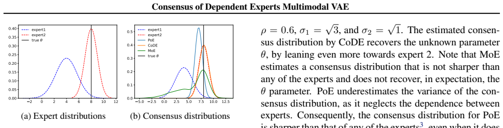
The paper's central claim is that a Bayesian posterior formed from expert point estimates, with a covariance matrix whose off-diagonal entries $\rho\sigma_i\sigma_j$ encode the dependence between expert errors, yields a correct consensus distribution for multimodal VAEs: $h(\theta_k|\mu_k) \sim \mathcal{N}(A_k^{-1}B_k, A_k^{-1})$ (Lemma 2). This posterior subsumes the product of experts when $\rho = 0$, leans toward more certain experts when $\rho > 0$, and avoids both the variance underestimation of product-of-experts and the vagueness of mixture-of-experts. Used inside a new ELBO that learns weights $\pi_k$ for each subset of modalities (Eq. 3), the method, CoDE-VAE, is shown empirically to improve the trade-off between generative coherence and generative quality, yield tighter log-likelihood estimates, and reduce the generative quality gap as more modalities are added, matching unimodal VAE quality in some cases.
Load-bearing premise
The paper assumes the joint error of all experts on every latent dimension is Gaussian with one shared correlation coefficient $\rho$ for every pair of experts and every dimension; if expert errors are not Gaussian, or their dependence is not captured by a single scalar, the CoDE posterior is misspecified and the reported gains may not hold.
Editorial extensions
If this is right
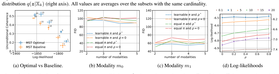
- CoDE-VAE reduces the generative quality gap as the number of modalities grows; with 4–5 PolyMNIST modalities its unconditional FID matches a unimodal VAE.
- Because it avoids modality sub-sampling, CoDE-VAE yields tighter log-likelihood estimates than mixture-of-experts methods such as mmJSD and MMVAE.
- The learned subset weights $\pi_k$ correlate with certainty: subsets with lower covariance trace receive larger weights, so the objective automatically up-weights reliable modality combinations.
- The CoDE posterior reduces to the product of experts when $\rho = 0$, so CoDE-VAE is a strict generalization of PoE-based multimodal VAEs.
- CoDE-VAE achieves classification accuracy comparable to leading multimodal VAEs, so modeling dependence does not hurt discriminative performance.
Reading between the lines
- Our inference: the single shared $\rho$ could be replaced by per-pair or per-dimension correlations (or learned), which might further improve the consensus posterior on heterogeneous modalities at the cost of more parameters and heavier cross-validation.
- Our inference: because CoDE only needs invertible $\Sigma_d$, negative or dimension-specific correlations are allowed; testing anti-correlated experts (e.g., complementary views) is a natural extension the authors do not explore.
- Our inference: the CoDE aggregation rule is not VAE-specific; it could be applied wherever expert distributions are combined, such as early-exit ensembles or LLM pairwise comparisons, as a drop-in replacement for product-of-experts.
- Our inference: the learned $\pi_k$ weights could double as a reliability signal for missing-modality inference, telling a deployed model which subset of available modalities to trust most.
Signed reviews
Editorial analysis
A structured set of objections, weighed in public.
Referee Report
Summary. The paper proposes CoDE (Consensus of Dependent Experts), a Bayesian method for aggregating single-modality variational posteriors in multimodal VAEs. The key idea is to model the joint error of the expert estimates as multivariate Gaussian with a covariance that encodes dependence through a single scalar correlation parameter ρ, then compute the consensus posterior via a conjugate Gaussian update (Lemma 2). The paper also introduces a weighted ELBO (Lemma 3) in which each subset-specific ELBO term is weighted by a learned categorical coefficient π_k, aiming to improve the coherence/quality trade-off and log-likelihood estimation relative to standard PoE/MoE baselines. Experiments on MNIST-SVHN-Text, PolyMNIST, and CUB report better balance between generative coherence and quality, tighter log-likelihoods, and a reduced generative quality gap. The manuscript includes proofs in appendices, ablations, and released code.
Significance. If the results hold, the paper makes a useful contribution to multimodal VAE inference: it provides a principled alternative to PoE/MoE that explicitly accounts for dependence among experts, subsumes PoE as a special case, and addresses the equal-weight limitation of the generalized multimodal ELBO. The mathematical core of Lemma 2 is a standard and correct conjugate Gaussian calculation, and the release of code supports reproducibility. However, the empirical claims are currently undermined by the evaluation protocol, which selects the method-specific parameter ρ and the reported architecture on the test set, and the derivation of Lemma 3 has a mathematical gap. These issues must be resolved before the practical significance of the method can be assessed.
major comments (3)
- [Section 4 and Appendix D.4] The reported empirical gains rely on test-set selection of the method-specific correlation parameter ρ and of the reported architecture. Section 4 states that 'all experiments present results that correspond to the ρ value demonstrating the strongest overall performance,' and Appendix D.4 reports that for PolyMNIST, 120 configurations per modality count were trained and 'the architecture with the smallest FID scores' was chosen. These selections are made on the same test set used for the headline numbers, and no equivalent test-set selection is applied to the baselines, which use their original implementations with their own optimal β. This protocol can only bias the comparison in favor of CoDE-VAE and does not support the central claim of an improved coherence/quality trade-off and tighter log-likelihoods. Please re-run the experiments using a held-out validation split to select ρ (and any architecture choices) and report results for the fixed validation-selected configuration.
- [Appendix A.3, Lemma 3] The proof of Lemma 3 contains an invalid algebraic step. The derivation begins with the sum of KL divergences and obtains an expression involving (2^M−1) log p(X); it then writes '∝ Σ E[...] + log p(X)' by 'factor[ing] out 2^M−1 as a constant.' Since log p(X) is the quantity being bounded, dropping the factor (2^M−1) is not a benign proportionality step for an inequality. As a consequence, the subsequent line 'logp(X) ≥ Σ E[...]' does not follow from the preceding equations. The claimed lower bound in Eq. (3) may still be valid with an appropriate constant (e.g., C = −K log K) and a proper derivation, but the proof as written is not correct. The authors should provide a complete derivation that explicitly handles the factor K and the constant C, or state the corrected bound.
- [Section 3.1, Lemma 1] The model assumes a single scalar correlation ρ shared by all pairs of experts and all latent dimensions, with off-diagonal entries σ_{i,j} = ρ σ_i σ_j in each Σ_d. This is a strong structural assumption about the error process of the encoders. The paper provides no diagnostic evidence that this assumption is adequate for the datasets considered; the sensitivity analyses in Table 12 and Fig. 6d vary only a global ρ, and no per-dimension or per-pair validation is reported. If the true error dependence is heterogeneous across dimensions or expert pairs, the CoDE posterior is misspecified and the reported improvements may not generalize. Please add an empirical check of the error covariance structure, or extend the parameterization to allow per-dimension or per-pair correlations, and discuss the effect of misspecification.
minor comments (6)
- [Section 4.2 and Fig. 4] There is a typo 'unonditional' in the title of the fourth panel of Fig. 4.
- [Appendix D.5] There is a typo: 'On the otter hand' should be 'On the other hand'.
- [Appendix D.4] The sentence about the authors' mmJSD results disagreeing with (Huang et al., 2022) references a paper on GAN-based image synthesis, which appears unrelated to mmJSD; the citation is likely incorrect and the comment should be removed or rephrased.
- [Appendix D.1] The entropy loss is scaled by a factor of 1,000, said to be 'found by cross-validation,' but no details are given about the validation procedure; since this scale directly influences the learned π and the overall objective, please specify how it was selected.
- [Appendix A.3] The citation to (Cormen et al., 2022) for the elementary fact E[ξ|Xk] = π_k is unnecessary and would be clearer as a direct statement.
- [Appendix E.1] The model name is inconsistently capitalized as 'CoDe-VAE' in one place; please use 'CoDE-VAE' consistently.
Circularity Check
No significant circularity: CoDE posterior and ELBO are derived from explicit assumptions; only evaluation-protocol concerns remain.
full rationale
Lemmas 1 and 2 form a standard Bayesian linear-Gaussian update: given expert point estimates mu and covariance Sigma, the posterior of theta is N(A^{-1}B, A^{-1}) with A = u^T Sigma^{-1} u and B = u^T Sigma^{-1} mu. This is derived in Appendix A.2 from the Gaussian error assumption and a flat prior; it does not define the target posterior in terms of the result. Remark 1 shows that PoE is recovered only in the rho=0 special case, so the dependence extension is a genuine generalization rather than a restatement. Lemma 3's ELBO is derived from KL decompositions in Appendix A.3; although the displayed inequality drops the factor 1/(2^M-1), that is a correctness concern in the proof, not a circular definition of log p(X). The only free parameter exclusive to CoDE-VAE is the scalar correlation rho, selected from a small grid; Section 4 states that results correspond to the rho value demonstrating the strongest overall performance, and Appendix D.4 selects the smallest-FID architecture among 120 configurations. This is a test-set-selection and fairness risk for the empirical comparison, but it is not a circular derivation: rho is a hyperparameter of the aggregation kernel, not a quantity obtained by inverting the final reported metric, and the reported numbers are actual generated-sample evaluations against external baselines. Self-citations (Mancisidor et al. 2024) appear only as related-work context and architecture-setting references, not as load-bearing support for the consensus formula. I therefore find no circular step.
Assumptions & free parameters
free parameters (3)
- rho (expert error correlation) =
cross-validated over [0, 0.2, 0.4, 0.6, 0.8]; selected values: 0.4 on MNIST-SVHN-Text, 0.4 on PolyMNIST, 0.6 on CelebA
- beta (KL regularization weight) =
cross-validated over [0.1,1,5,10,15,20]; e.g., beta=5 on MNIST-SVHN-Text for CoDE-VAE
- Entropy loss scale =
1000
assumptions (5)
- domain assumption Gaussian error model for expert estimates (Lemma 1)
- domain assumption Flat prior on the consensus parameter θ_k (Lemma 2)
- domain assumption Conditional independence of modalities given z (Section 3)
- domain assumption Mean-field factorization q(z,ξ|X_k)=q(z|X_k)q(ξ|X_k) (Appendix A.3)
- ad hoc to paper Single shared nonnegative correlation rho for all expert pairs and dimensions
Cite this review
Pith. "Pith review of Aggregation of Dependent Expert Distributions in Multimodal Variational Autoencoders." pith.science (2026). https://pith.science/paper/MDSNDOHV
@misc{pith2026250501134,
  author       = {Pith},
  title        = {Pith review of: Aggregation of Dependent Expert Distributions in Multimodal Variational Autoencoders},
  year         = {2026},
  howpublished = {\url{https://pith.science/paper/MDSNDOHV}},
  note         = {Machine review of arXiv:2505.01134}
}
read the original abstract
Multimodal learning with variational autoencoders (VAEs) requires estimating joint distributions to evaluate the evidence lower bound (ELBO). Current methods, the product and mixture of experts, aggregate single-modality distributions assuming independence for simplicity, which is an overoptimistic assumption. This research introduces a novel methodology for aggregating single-modality distributions by exploiting the principle of consensus of dependent experts (CoDE), which circumvents the aforementioned assumption. Utilizing the CoDE method, we propose a novel ELBO that approximates the joint likelihood of the multimodal data by learning the contribution of each subset of modalities. The resulting CoDE-VAE model demonstrates better performance in terms of balancing the trade-off between generative coherence and generative quality, as well as generating more precise log-likelihood estimations. CoDE-VAE further minimizes the generative quality gap as the number of modalities increases. In certain cases, it reaches a generative quality similar to that of unimodal VAEs, which is a desirable property that is lacking in most current methods. Finally, the classification accuracy achieved by CoDE-VAE is comparable to that of state-of-the-art multimodal VAE models.
Figures


Figures from the paper (17 more)






Reference graph
Works this paper leans on
-
[1]
logp(X) ∝ X Xk Eq(z,ξ|Xk) log q(z,ξ|Xk) p(X|z)p(z)p(ξ) + logp(X), where in line 3 we factor out 2M− 1 as a constant, which should not affect the optimization (Wu & Goodman, 2019). Assuming a categorical prior distribution for p(ξ) with probability mass function η = (1/K,··· , 1/K), where K = 2M− 1, i.e. equal prior probabilities for all subsets, we obtain...
work page 2019
-
[2]
Finally, all experiments report the average performance and standard deviations of 3 different runs and for the benchmark models we use the following original implementation codes: MMV AE https://github.com/iffsid/mmvae/tree/public; MV AE, mmJSD, and MoPoE https://github.com/thomassutter/MoPoE; MVT- CAE https://github.com/gr8joo/MVTCAE/tree/master; MMV AE...
work page 2022
-
[4]
The last column for each model specifies the kernel size, stride, padding, and dilation
SVHN encoder and decoder layers. The last column for each model specifies the kernel size, stride, padding, and dilation. All layers are 2D convolutional (conv) and upconvolutional (upconv) in the encoder and decoder, respectively, with ReLU activations. Finally, the number of input and output dimensions in each layer is shown in the columns #F.In and #F....
work page 2020
-
[5]
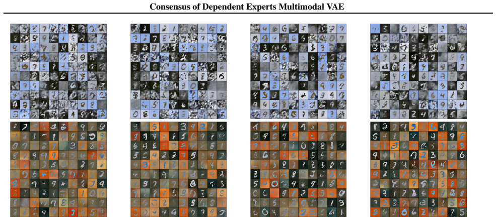
(bottom row). In Fig. 12, we show random generated digits corresponding to modality 1 (top row) and modality 2 (bottom row), as a function of the number of modalities in the dataset, i.e. the first column shows generated images with a CoDE-V AE model trained with 2 modalities, while the last column shows images generated with a model trained with 5 modali...
work page 2019
-
[6]
Therefore, forρ = 0 the CoDE parameters are simply PoE parameters
Hence, Σ = σ2 1 0 0 σ2 2 , Σ−1 = 1 σ2 1σ2 2 σ2 2 0 0 σ2 1 = 1/σ2 1 0 0 1 /σ2 2 , A =τ1,1 +τ2,2,B =τ1,1µ1 +τ2,2µ2, and the consensus distribution isq(z|x1,x 2)∼N τ1,1µ1+τ2,2µ2 τ1,1+τ2,2 , 1 τ1,1+τ2,2 , where τi = 1/σ2 i , like in (Wu & Goodman, 2018). Therefore, forρ = 0 the CoDE parameters are simply PoE parameters. As shown by (Winkler, 1981), we can wri...
work page 2018
-
[7]
Models are trained on single A100 GPUs with AMD EPYC Milan processors with 24 cores
is used on all datasets. Models are trained on single A100 GPUs with AMD EPYC Milan processors with 24 cores. We find the optimal correlation parameterρ by cross-validation using the values [0, 0.2, 0.4, 0.6, 0.8] and the off-diagonal in the covariance matrices Σd in Lemma 1 are specified as σj,i = ρσjσi. We cross-validate only positive ρ values, as it is...
work page 2016
-
[8]
The last column for each model specifies the kernel size, stride, padding, and dilation
PolyMNIST encoder and decoder layers. The last column for each model specifies the kernel size, stride, padding, and dilation. All layers are 2D convolutional (conv) and upconvolutional (upconv) in the encoder and decoder, respectively, with ReLU activations. Finally, the number of input and output dimensions in each layer is shown in the columns #F.In an...
-
[11]
MV AE MMV AE mmJSD MoPoE-V AE MVTCAE MMV AE+ CoDE-V AE β 5 0.1 5 10 20 5 5 ρ 0.4 D.4
Optimal parameters for all models in the classification on MNIST-SVHN-Text data. MV AE MMV AE mmJSD MoPoE-V AE MVTCAE MMV AE+ CoDE-V AE β 5 0.1 5 10 20 5 5 ρ 0.4 D.4. P OLYMNIST Data and training details: the PolyMNIST dataset is built upon MNIST by varying the original background. A random 28x28 crop from 5 different images is used as the background to f...
work page 2021
Show all 18 references
-
[13]
The decoders are conditioned on representations from the prior (top row) and the consensus distributionq(z|X = 5)
Random generation of digits for all modalities. The decoders are conditioned on representations from the prior (top row) and the consensus distributionq(z|X = 5). • 3 modalities →{m0,m1,m2} • 4 modalities →{m0,m1,m2,m3} • 5 modalities →{m0,m1,m2,m3,m4} Given that we cross-vali...
2022
-
[14]
The conditional generations by CoDE-V AE are based on the full subsets
The top row shows random generations by unimodal V AE, while the bottom row corresponds to generations by CoDE-V AE. The conditional generations by CoDE-V AE are based on the full subsets. brown, black}. Then, for each of the eight captions, we generate ten images (eighty in t...
2020
-
[16]
The average is calculated over all subsets in each case, i.e
Average coherence and classification accuracy as a function of correlation ρ, obtained with CoDE-V AE models trained with 2, 3, 4, and 5 modalities. The average is calculated over all subsets in each case, i.e. 3, 7, 15, and 31 subsets, respectively. for the image modality ple...
2022
-
[20]
6800 6600 6400 6200 6000 5800 Log-likelihood 0.1 0.2 0.3 0.4 0.5Unconditional Coherence 0.10.1 11 55 10 10 1515 2020 PolyMNIST Optimal PolyMINST Baseline Figure
Trade-off between generative coherence (↑) and generative quality (↓) forβ∈ [1, 2.5, 5] on the PolyMNIST dataset. 6800 6600 6400 6200 6000 5800 Log-likelihood 0.1 0.2 0.3 0.4 0.5Unconditional Coherence 0.10.1 11 55 10 10 1515 2020 PolyMNIST Optimal PolyMINST Baseline Figure
-
[2017]
Cross-modal Variational Align- ment of Latent Spaces
Theodoridis, T., Chatzis, T., Solachidis, V ., Dimitropou- los, K., and Daras, P. Cross-modal Variational Align- ment of Latent Spaces. In 2020 IEEE/CVF Conference on Computer Vision and Pattern Recognition Workshops (CVPRW), pp. 4127–4136, Seattle, W A, USA,
2020
-
[2018]
The caltech-ucsd birds-200-2011 dataset
Wah, C., Branson, S., Welinder, P., Perona, P., and Be- longie, S. The caltech-ucsd birds-200-2011 dataset
2011
-
[2020]
Effi- cient llm comparative assessment: a product of experts framework for pairwise comparisons
Liusie, A., Raina, V ., Fathullah, Y ., and Gales, M. Effi- cient llm comparative assessment: a product of experts framework for pairwise comparisons. arXiv preprint arXiv:2405.05894,
-
[2021]
We assume Laplace likelihoods
and not in (Daunhawer et al., 2022). We assume Laplace likelihoods. The dimensionality of the latent representations is set to 512 as in (Sutter et al., 2021; Daunhawer et al., 2022; Palumbo et al., 2023). The results in Fig. 4 are based on all 5 modalities of the PolyMNIST da...
2022
-
[2022]
Deep Residual Learning for Image Recognition
He, K., Zhang, X., Ren, S., and Sun, J. Deep Residual Learning for Image Recognition. In 2016 IEEE Con- ference on Computer Vision and Pattern Recognition (CVPR), pp. 770–778,
2016
-
[2023]
That is, divide the total number of dimensions in the latent space assumed by models without modality-specific variables by the number of modalities
to select the dimension of the modality-specific latent space in MMV AE+. That is, divide the total number of dimensions in the latent space assumed by models without modality-specific variables by the number of modalities. We use weights to scale the decoder networks, as the ...
2021
Reviewed August 16, 2026 · model on record in the stance chip above.
Discussion (0). Continue with ORCID to comment.