REVIEW 4 major objections 5 minor 53 references
Modeling and Optimization with Gaussian Processes in Reduced Eigenbases -- Extended Version
T0 review · 4 major / 5 minor · reviewed 2026-08-14 · deepseek-v4-flash
Pith's one-line read The paper argues that building Gaussian-process surrogates in a PCA-derived eigenshape basis gives more accurate models and faster optimization than building them in the original CAD parameter basis, at low evaluation budgets.
desk verdict A solid, honest methods paper whose modeling claims hold up, but the optimization branch needs pre-image diagnostics and sensitivity analysis before I'd fully trust the headline gains. read the letter →
The pith
A machine-rendered reading of the paper's core claim, the machinery that carries it, and where it could break.
The reading
What carries the argument
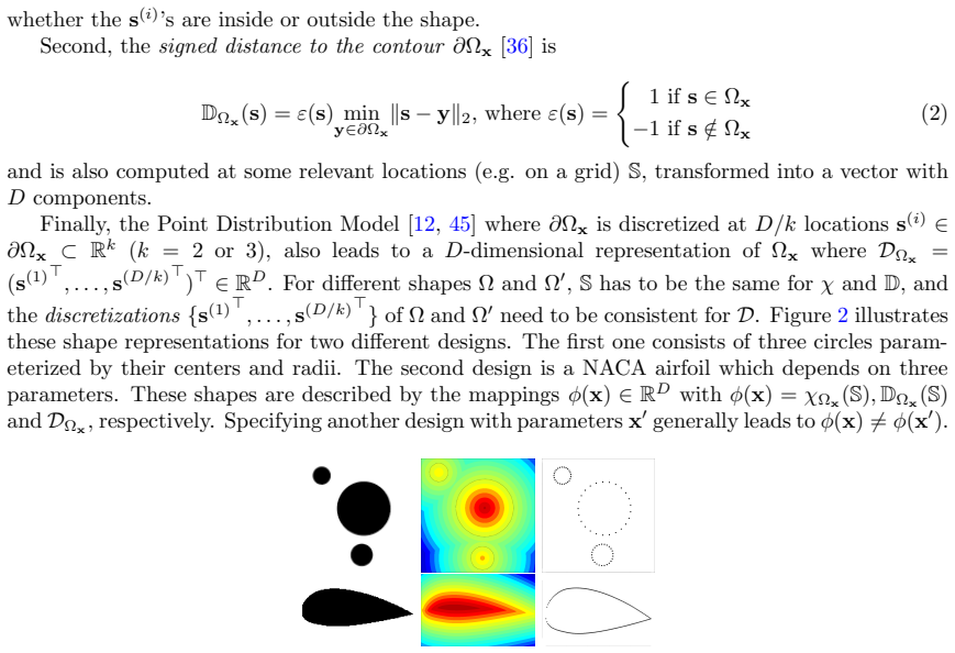
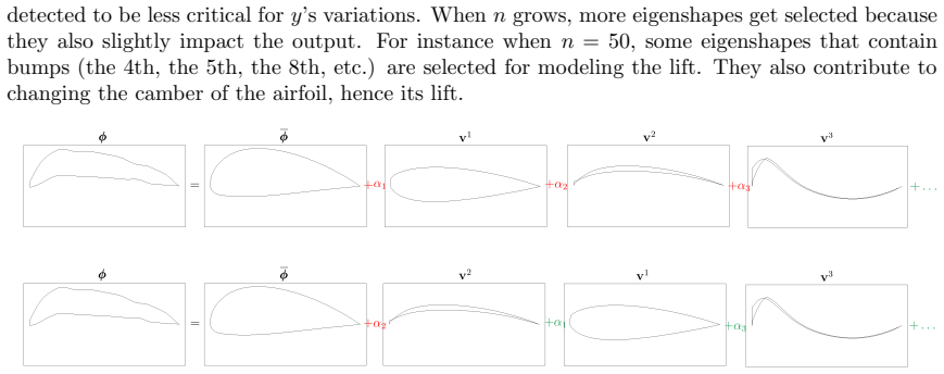
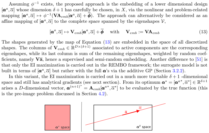
The load-bearing machinery is a chain of four objects. First, a high-dimensional shape mapping $\varphi(x)$ — in this paper the discretization of the contour, not the characteristic function or signed distance — gives a representation space in which PCA eigenvalues drop to zero at the true effective dimension and the eigenvectors $v_j$ are interpretable "eigenshapes." Second, an $L_1$-penalized concentrated log-likelihood selects the active eigenshape components $\alpha_a$ by driving inverse length-scales to zero; this is the supervised step that prevents geometric modes irrelevant to the output from dominating the surrogate. Third, the additive GP $Y(\alpha)=\beta+Y_a(\alpha_a)+Y_{\bar a}(\alpha_{\bar a})$ splits the fit into an anisotropic GP on $\alpha_a$ and an isotropic GP on the inactive components $\alpha_{\bar a}$, keeping the number of learned hyperparameters small enough for $n\ll D$. Fourth, optimization couples expected improvement maximization in $\alpha_a$ with a random embedding along one line in $\alpha_{\bar a}$, and the pre-image problem together with the replication strategy ties proposed eigen-coordinates back to evaluable CAD parameters without letting repeated off-manifold proposals fool the surrogate.
What would settle it
Run the full pipeline on a parametric family where the map from eigenshape coefficients back to shapes is known to be poor, such as shapes with many independent local bumps that create a highly non-convex or high-dimensional manifold; if the distance $\|\alpha^{(n+1)*}-\alpha(x^{(n+1)})\|$ does not decay as the budget grows and the additive eigenshape GP's best value stays worse than a CAD-parameter GP at equal budget, the central claim fails.
Extended reading notes
Core claim
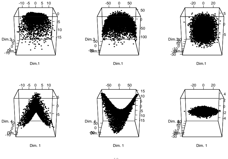
The paper's central claim is that the effective coordinates for shape surrogate modeling and optimization are the PCA coefficients $\alpha = V^\top(\varphi(x)-\bar\varphi)$ of a discretized contour representation, and that the objective's variation is concentrated on a small subset of these coordinates. To exploit this, the authors maximize an $L_1$-penalized GP log-likelihood to declare a subset $\alpha_a$ of eigenshape components active, and model $Y(\alpha)=\beta+Y_a(\alpha_a)+Y_{\bar a}(\alpha_{\bar a})$, an additive GP with an anisotropic kernel on the active components and an isotropic kernel on the inactive ones. Optimization maximizes expected improvement over $\alpha_a$ together with a random direction in the inactive space, solves the pre-image problem $x^{(n+1)}=\arg\min_x\|\varphi(x)-\bar\varphi-V\alpha^{(n+1)*}\|^2$ to obtain an evaluable design, and, when the proposed $\alpha^*$ is far from the recovered $\alpha(x)$, updates the GP with both points ("replication"). Across all benchmark problems, including a CFD NACA airfoil, the additive eigenshape GP with this acquisition strategy yields higher $R^2$ and lower objective values at low budgets than a GP built directly in the CAD parameters $x$.
Load-bearing premise
The load-bearing premise is that the pre-image problem can be solved well enough: the CAD parameters recovered from a proposed eigenshape vector must produce a shape whose actual eigen-coordinates are close to the proposed ones, otherwise the GP is updated at points the acquisition function did not choose and replicated data mislead the surrogate.
Editorial extensions
If this is right
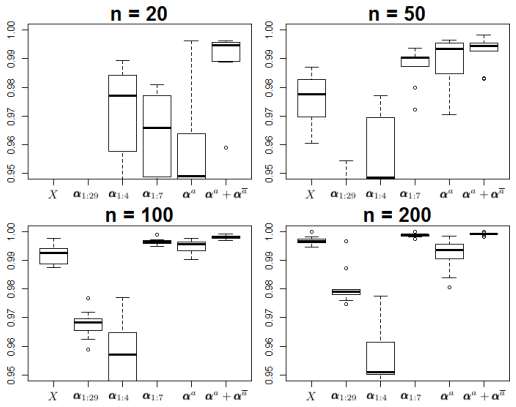
- At evaluation budgets of 20 to 200 calls, the additive eigenshape GP gives higher prediction $R^2$ than a GP in the CAD parameter space on every benchmark tested, including a CFD airfoil with 22 parameters.
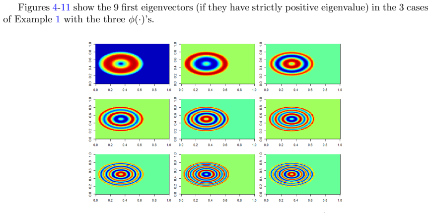
- When the first eigenshapes do not affect the objective (as in the rectangle case), selecting active components by penalized likelihood avoids the failure mode of truncating to the first principal components.
- Optimizing expected improvement in the active subspace plus a random line in the inactive subspace reaches lower objective values in fewer calls than optimizing over all variables or only active variables.
- Replicating the objective value at off-manifold proposed points removes their acquisition uncertainty and prevents the optimizer from repeatedly proposing the same unreachable shape.
- The method's advantage is largest at small budgets: as the number of evaluations grows, higher-dimensional eigenshape models catch up, so the claim is specifically about early-stage optimization.
Reading between the lines
- Inference: Because the method only requires a fast auxiliary map $\varphi$ and a database of plausible inputs, it should transfer to any high-dimensional input whose output is governed by a low-dimensional geometric description, such as images, signals, or material microstructures, not just CAD contours.
- Inference: The replication strategy suggests a general principle for latent-space Bayesian optimization: whenever the acquisition maximizer cannot be exactly realized, add the virtual observation at the proposed latent point; the paper's experiments indicate this improves exploration but do not prove it in general.
- Inference: If the observed near-convexity of the eigenshape manifold for contour discretizations holds more generally, the pre-image projection would be unique and the whole loop could be accelerated; proving or disproving convexity of $\mathcal{A}$ is a testable mathematical question.
Signed reviews
Editorial analysis
A structured set of objections, weighed in public.
Referee Report
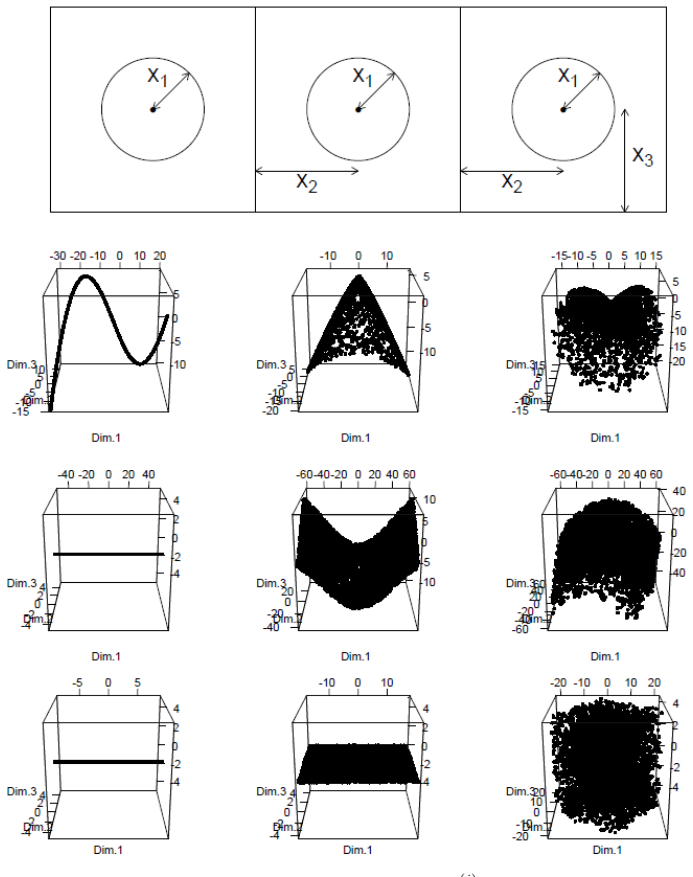
Summary. The paper proposes an end-to-end method for Bayesian optimization of expensive parametric shape functions. CAD shapes are represented by high-dimensional discretizations φ(x); a PCA on a large database of such representations yields an eigenshape coordinate system α; an L1-penalized GP likelihood selects a small set of output-relevant active coordinates αa; an additive GP with an anisotropic kernel over αa and an isotropic kernel over the remaining coordinates models the objective; and expected improvement is maximized over the active coordinates plus a random line in the inactive coordinates. The EI maximizer is mapped back to CAD parameters by solving the pre-image problem (Eq. 16), and a replication strategy adds a virtual point at the off-manifold EI maximizer. The paper reports R² comparisons on four benchmarks (Tables 11–14), optimization comparisons on the catenoid and rectangular-heart problems (Tables 15–17), and two NACA 22 airfoil runs (Figures 40–41). The abstract claims that at low budgets the methodology delivers a more accurate model and faster optimization than working directly with the CAD parameters.
Significance. The central claim is practically valuable and, for the metamodeling branch, largely supported: the additive GP achieves the best R² on every benchmark, test sets are independent, and the authors honestly report cases where unsupervised dimension reduction fails (e.g., GP(α1:2) on the heart problem). The optimization experiments also show consistent gains for the additive GP with embedding and replication on the catenoid and heart problems. If the pre-image accuracy issue is resolved, the method is a useful contribution to high-dimensional shape optimization, since the shape mapping and PCA are cheap compared with simulator calls. The paper does not ship code or data, but the analytic benchmarks are specified in enough detail to be reproducible.
major comments (4)
- [Section 4.2, Eq. (16)] The optimization branch of the central claim rests on the pre-image step, but its quality is never measured. The EI maximizer α* selects a shape in eigenspace; the evaluated point is x* = argmin ‖φ(x)−(Vα*+φ̄)‖, and the GP is updated at α(x*) and possibly at the virtual point (α*, f(x*)). If ‖φ(x*)−(Vα*+φ̄)‖ is comparable to the GP length scales, the acquisition evaluates a different point than intended and replication teaches the surrogate a value at an unattainable coordinate. The manuscript only says that solving Eq. (16) is 'relatively not costly' and never reports the achieved residual, the optimizer and bounds used for Eq. (16), the fraction of iterations with α* outside the manifold, or the distance between α(x*) and α* during optimization. These diagnostics should be provided for Tables 16–17 and the NACA runs; if the residuals turn out to be non-negligible, the comparison between replication and no replication needs to be revisited.
- [Section 3.2.1, Definition 1] The active-set procedure depends on several hyperparameters that are set once without sensitivity analysis: the L1 weight λ = n/D in Eq. (8), the factor 10 in Definition 1, and the eigenvalue-truncation criterion for d′ in Section 2.3 (the text gives '99.9, 99.95 or 99.99%' without stating the value used in each benchmark). Since the additive model's performance and the EI embedding dimension are driven by the selected active set, the central comparisons in Tables 12–14 and 16–17 could partly reflect these choices. A sensitivity study over reasonable ranges of λ and the active threshold, reporting both R² and optimization traces, would let the reader assess robustness.
- [Section 4.2, Definition 2] Replication is presented as a constant prolongation of the surrogate outside the manifold, but the validity of that prolongation is an assumption rather than a demonstrated fact. The only evidence is the aggregate improvement in Table 16 (26.19 with replication versus 27.58 without). If the pre-image residual is large, the replicated point (α*, f(x*)) is a false observation at an unattainable coordinate and can bias the GP. The threshold d0 in Definition 2, the minimal pairwise distance among the 5000 database shapes, is likewise not related to GP length scales and can strongly affect replication frequency. Please provide, for the experiments of Table 16, the distribution of ‖φ(x*)−(Vα*+φ̄)‖, the fraction of replication events, and a comparison against an alternative that updates only at the projected point but avoids repeated sampling of the same α* region; this would isolate the benefit of the virtual point from the benefit of variance reduction at α*.
- [Section 4.3.2, Figures 40–41] The engineering demonstration on the NACA 22 airfoil consists of only two runs per objective, and the two algorithms use different initial-design sizes (10 initial points for AddGP(αa+ᾱa)-EI embed versus 50 for GP(X)-EI(X)). With two runs and a confounded initialization budget, the 'faster optimization' conclusion for the realistic CFD case is not statistically established. I recommend either more repeats, possibly on a cheaper surrogate of the CFD code, or explicit framing of the NACA results as an illustrative case study rather than as support for the general claim.
minor comments (5)
- [Section 2.3.1] The text states, 'Without formal proof, we think that this is related to the observed property that the d first eigencomponents … make a convex set'; since convexity is relevant to the projection discussion in Section 4.2, this conjecture should be either proven, cited, or explicitly marked as non-essential.
- [Section 3.2.1] The passages 'Numerical experiments not reported here for reasons of brevity…' and 'In experiments that are not reported here…' assert robustness properties (local optima of the penalized likelihood, behavior with normalized αj's) without evidence; these claims should be removed or the supporting experiments reported in an appendix.
- [Section 2.1, Tables 1–5] The signed-distance function and the contour discretization are both denoted D, which makes headings such as 'Signed Distance Discretization' ambiguous; using distinct symbols such as D_SD and D_cont would improve readability.
- [Section 4.1] The one-dimensional embedding coordinate α and the inactive vector ᾱa are visually similar, and the Kronecker symbol δ overlaps with the active dimension δ; a different symbol for the embedding coordinate would reduce confusion.
- [Section 1 and Definition 1] There are typographical artifacts such as 'a vector ofd Computer Aided Design' in Section 1 and an unbalanced parenthesis in Definition 1 ('and{ααα(1:n), y(1:n))}'); a careful proofread is needed.
Circularity Check
No significant circularity: eigenshape GP claims are validated on held-out data, and the only self-citations are non-load-bearing.
full rationale
The paper's central claim is that, at low budgets, a GP built in the eigenshape basis with supervised active-dimension selection, random-embedding EI maximization, and the replication strategy is more accurate and faster than a GP built directly on CAD parameters. Nothing in the derivation reduces to the claim by construction. The PCA basis is computed from the cheap shape mapping φ without using objective values; the active eigenshapes are chosen by L1-penalized likelihood on the observed training responses; and all predictive and optimization comparisons (Tables 11-17, Figures 40-41) are made on distinct test sets or independent runs. No fitted parameter is relabeled as a prediction. The only self-references are the opening footnote identifying the extended version of the authors' own SMO 2020 article and reference [21], which is a different Gaudrie et al. work; neither carries a load-bearing premise, and no uniqueness theorem or prior self-citation is invoked to force the method choice. The nearest thing to an unverified assumption is the pre-image problem (Eq. 16): its residual is never reported, so the replication gain, e.g. 26.19 vs 27.28 in Table 16, could be sensitive to how accurately EI maximizers project back to attainable shapes. That is a correctness and robustness risk about an implementation detail, not a circular step in the derivation. The conclusion that eigenshape coordinates are more relevant than CAD parameters for these problems is an empirical finding supported by the held-out experiments rather than an input to their construction.
Assumptions & free parameters
free parameters (5)
- L1 penalization weight λ =
λ = n/D
- Variance threshold for retaining eigenshapes =
Examples use 0.95, 0.99, or manual choices (2,3,4,6,7,16,20)
- Active dimension factor =
10
- Replication distance threshold =
d0 = min pairwise distance in Φ database
- Number of shapes in PCA database =
N = 5000
assumptions (5)
- domain assumption The most significant shape variations (largest PCA eigenvalues) are responsible for the largest output variations.
- domain assumption The objective function f varies smoothly enough in the eigenshape coordinates for a stationary GP with a Matérn or squared-exponential kernel to be appropriate.
- ad hoc to paper The additive decomposition Y(α) = β + Ya(αa) + Yā(αā) with independent kernels is a valid structural model for f.
- domain assumption The manifold A of valid α's is well approximated by the empirical manifold A_N and lies inside its covering hyper-rectangle.
- ad hoc to paper Replicating the output f(x) at the non-real design α* (constant prolongation outside A) does not bias the surrogate.
Cite this review
Pith. "Pith review of Modeling and Optimization with Gaussian Processes in Reduced Eigenbases -- Extended Version." pith.science (2026). https://pith.science/paper/MKWH7HLH
@misc{pith2026190811272,
  author       = {Pith},
  title        = {Pith review of: Modeling and Optimization with Gaussian Processes in Reduced Eigenbases -- Extended Version},
  year         = {2026},
  howpublished = {\url{https://pith.science/paper/MKWH7HLH}},
  note         = {Machine review of arXiv:1908.11272}
}
read the original abstract
Parametric shape optimization aims at minimizing an objective function f(x) where x are CAD parameters. This task is difficult when f is the output of an expensive-to-evaluate numerical simulator and the number of CAD parameters is large. Most often, the set of all considered CAD shapes resides in a manifold of lower effective dimension in which it is preferable to build the surrogate model and perform the optimization. In this work, we uncover the manifold through a high-dimensional shape mapping and build a new coordinate system made of eigenshapes. The surrogate model is learned in the space of eigenshapes: a regularized likelihood maximization provides the most relevant dimensions for the output. The final surrogate model is detailed (anisotropic) with respect to the most sensitive eigenshapes and rough (isotropic) in the remaining dimensions. Last, the optimization is carried out with a focus on the critical dimensions, the remaining ones being coarsely optimized through a random embedding and the manifold being accounted for through a replication strategy. At low budgets, the methodology leads to a more accurate model and a faster optimization than the classical approach of directly working with the CAD parameters.
Figures

Figures from the paper (38 more)













Reference graph
Works this paper leans on
-
[1]
Anisotropy models for spatial data
Denis Allard, Rachid Senoussi, and Emilio Porcu. Anisotropy models for spatial data. Math- ematical Geosciences, 48(3):305–328, 2016
work page 2016
-
[2]
Performance evaluation of an advanced local search evo- lutionary algorithm
Anne Auger and Nikolaus Hansen. Performance evaluation of an advanced local search evo- lutionary algorithm. In Congress on evolutionary computation , volume 2, pages 1777–1784. IEEE, 2005
work page 2005
-
[3]
Adaptive control processes: a guided tour
Richard E Bellman. Adaptive control processes: a guided tour . Princeton university press, 1961
work page 1961
-
[4]
Sequential dimension reduction for learning features of expensive black-box functions
Malek Ben Salem, Fran¸ cois Bachoc, Olivier Roustant, Fabrice Gamboa, and Lionel Tomaso. Sequential dimension reduction for learning features of expensive black-box functions. 2018
work page 2018
-
[5]
The proper orthogonal decomposition in the analysis of turbulent flows
Gal Berkooz, Philip Holmes, and John L Lumley. The proper orthogonal decomposition in the analysis of turbulent flows. Annual review of fluid mechanics , 25(1):539–575, 1993
work page 1993
-
[6]
A warped kernel improving ro- bustness in Bayesian optimization via random embeddings
Micka¨ el Binois, David Ginsbourger, and Olivier Roustant. A warped kernel improving ro- bustness in Bayesian optimization via random embeddings. In International Conference on Learning and Intelligent Optimization , pages 281–286. Springer, 2015
work page 2015
-
[7]
On the choice of the low-dimensional domain for global optimization via random embeddings
Micka¨ el Binois, David Ginsbourger, and Olivier Roustant. On the choice of the low-dimensional domain for global optimization via random embeddings. arXiv preprint arXiv:1704.05318 , 2017
work page Pith review arXiv 2017
-
[8]
Mohamed Amine Bouhlel, Nathalie Bartoli, Abdelkader Otsmane, and Joseph Morlier. Im- proving kriging surrogates of high-dimensional design models by partial least squares dimension reduction. Structural and Multidisciplinary Optimization , 53(5):935–952, 2016
work page 2016
Show all 53 references
-
[9]
Investigation of adaptive design variables bounds in dimensionality reduction for aerodynamic shape optimization
Davide Cinquegrana and Emiliano Iuliano. Investigation of adaptive design variables bounds in dimensionality reduction for aerodynamic shape optimization. Computers & Fluids, 174:89– 109, 2018
2018
-
[10]
Shapes of embedded minimal surfaces
Tobias H Colding and William P Minicozzi. Shapes of embedded minimal surfaces. Proceedings of the National Academy of Sciences , 103(30):11106–11111, 2006
2006
-
[11]
Active subspace methods in theory and practice: applications to kriging surfaces
Paul Constantine, Eric Dow, and Qiqi Wang. Active subspace methods in theory and practice: applications to kriging surfaces. SIAM Journal on Scientific Computing , 36(4):A1500–A1524, 2014
2014
-
[12]
Active shape models-their training and application
Timothy F Cootes, Christopher J Taylor, David H Cooper, and Jim Graham. Active shape models-their training and application. Computer vision and image understanding , 61(1):38–59, 1995. 57
1995
-
[13]
Statistics for spatial data
Noel Cressie. Statistics for spatial data. Terra Nova, 4(5):613–617, 1992
1992
-
[14]
Package ‘kergp’
Yves Deville, David Ginsbourger, Nicolas Durrande, and Olivier Roustant. Package ‘kergp’. 2015
2015
-
[15]
´Etude de classes de noyaux adapt´ ees ` a la simplification et ` a l’interpr´ etation des mod` eles d’approximation
Nicolas Durrande. ´Etude de classes de noyaux adapt´ ees ` a la simplification et ` a l’interpr´ etation des mod` eles d’approximation. Une approche fonctionnelle et probabiliste. PhD thesis, ´Ecole Nationale Sup´ erieure des Mines de Saint-´Etienne, 2011
2011
-
[16]
Additive covariance kernels for high-dimensional Gaussian process modeling
Nicolas Durrande, David Ginsbourger, and Olivier Roustant. Additive covariance kernels for high-dimensional Gaussian process modeling. In Annales de la Facult´ e des sciences de Toulouse: Math´ ematiques, volume 21, pages 481–499, 2012
2012
-
[17]
Additive Gaussian processes
David Duvenaud, Hannes Nickisch, and Carl Edward Rasmussen. Additive Gaussian processes. In Advances in neural information processing systems , pages 226–234, 2011
2011
-
[18]
Recent advances in surrogate-based optimization
Alexander IJ Forrester and Andy J Keane. Recent advances in surrogate-based optimization. Progress in aerospace sciences, 45(1-3):50–79, 2009
2009
-
[19]
A statistical view of some chemometrics regression tools
Ildiko E Frank and Jerome Friedman. A statistical view of some chemometrics regression tools. Technometrics, 35(2):109–135, 1993
1993
-
[20]
An algorithm for finding intrinsic dimensionality of data
Keinosuke Fukunaga and David R Olsen. An algorithm for finding intrinsic dimensionality of data. IEEE Transactions on Computers , 100(2):176–183, 1971
1971
-
[21]
Budgeted multi-objective optimization with a focus on the central part of the Pareto front- extended version
David Gaudrie, Rodolphe Le Riche, Victor Picheny, Benoit Enaux, and Vincent Herbert. Budgeted multi-objective optimization with a focus on the central part of the Pareto front- extended version. arXiv preprint arXiv:1809.10482 , 2018
2018 arXiv
-
[22]
Principal component analysis
Ian Jolliffe. Principal component analysis. Springer, 2011
2011
-
[23]
A taxonomy of global optimization methods based on response surfaces
Donald R Jones. A taxonomy of global optimization methods based on response surfaces. Journal of global optimization , 21(4):345–383, 2001
2001
-
[24]
Efficient Global Optimization of expensive black-box functions
Donald R Jones, Matthias Schonlau, and William J Welch. Efficient Global Optimization of expensive black-box functions. Journal of Global optimization , 13(4):455–492, 1998
1998
-
[25]
A data-based approach for fast airfoil analysis and optimization
Jichao Li, Mohamed Amine Bouhlel, and Joaquim Martins. A data-based approach for fast airfoil analysis and optimization. In 2018 AIAA/ASCE/AHS/ASC Structures, Structural Dy- namics, and Materials Conference , page 1383, 2018
2018
-
[26]
Surrogate-based aerodynamic shape optimization with the active subspace method
Jichao Li, Jinsheng Cai, and Kun Qu. Surrogate-based aerodynamic shape optimization with the active subspace method. Structural and Multidisciplinary Optimization , 59(2):403–419, 2019
2019
-
[27]
On the limited memory BFGS method for large scale optimiza- tion
Dong Liu and Jorge Nocedal. On the limited memory BFGS method for large scale optimiza- tion. Mathematical programming, 45(1-3):503–528, 1989
1989
-
[28]
Choosing the sample size of a computer experiment: A practical guide
Jason L Loeppky, Jerome Sacks, and William J Welch. Choosing the sample size of a computer experiment: A practical guide. Technometrics, 51(4):366–376, 2009. 58
2009
-
[29]
Genetic optimization using derivatives: the rgenoud package for R
Walter R Mebane Jr, Jasjeet S Sekhon, et al. Genetic optimization using derivatives: the rgenoud package for R. Journal of Statistical Software , 42(11):1–26, 2011
2011
-
[30]
Kernel PCA and de-noising in feature spaces
Sebastian Mika, Bernhard Sch¨ olkopf, Alexander Smola, Klaus-Robert M¨ uller, Matthias Scholz, and Gunnar R¨ atsch. Kernel PCA and de-noising in feature spaces. In Advances in neural information processing systems, pages 536–542, 1999
1999
-
[31]
On Bayesian methods for seeking the extremum
Jonas Mockus. On Bayesian methods for seeking the extremum. In Optimization Techniques IFIP Technical Conference, pages 400–404. Springer, 1975
1975
-
[32]
Test functions for optimization needs
Marcin Molga and Czes law Smutnicki. Test functions for optimization needs. Test functions for optimization needs, 101, 2005
2005
-
[33]
Kriging surrogate model with co- ordinate transformation based on likelihood and gradient
Nobuo Namura, Koji Shimoyama, and Shigeru Obayashi. Kriging surrogate model with co- ordinate transformation based on likelihood and gradient. Journal of Global Optimization , 68(4):827–849, 2017
2017
-
[34]
On the accuracy of kriging model in active subspaces
Pramudita S Palar and Koji Shimoyama. On the accuracy of kriging model in active subspaces. In 2018 AIAA/ASCE/AHS/ASC Structures, Structural Dynamics, and Materials Conference , page 0913, 2018
2018
-
[35]
Towards a space re- duction approach for efficient structural shape optimization
Balaji Raghavan, Piotr Breitkopf, Yves Tourbier, and Pierre Villon. Towards a space re- duction approach for efficient structural shape optimization. Structural and Multidisciplinary Optimization, 48(5):987–1000, 2013
2013
-
[36]
Numerical assessment of springback for the deep drawing process by level set interpolation using shape manifolds
Balaji Raghavan, Guenhael Le Quilliec, Piotr Breitkopf, Alain Rassineux, Jean-Marc Roelandt, and Pierre Villon. Numerical assessment of springback for the deep drawing process by level set interpolation using shape manifolds. International journal of material forming , 7(4):48...
2014
-
[37]
Gaussian Processes for Machine Learn- ing
Carl Edward Rasmussen and Christopher KI Williams. Gaussian Processes for Machine Learn- ing. The MIT Press, 2006
2006
-
[38]
DiceKriging, DiceOptim: Two R packages for the analysis of computer experiments by kriging-based metamodeling and opti- mization
Olivier Roustant, David Ginsbourger, and Yves Deville. DiceKriging, DiceOptim: Two R packages for the analysis of computer experiments by kriging-based metamodeling and opti- mization. 2012
2012
-
[39]
Design and analysis of computer experiments
Jerome Sacks, William J Welch, Toby J Mitchell, and Henry P Wynn. Design and analysis of computer experiments. Statistical science, pages 409–423, 1989
1989
-
[40]
Sensitivity analysis in practice: a guide to assessing scientific models
Andrea Saltelli, Stefano Tarantola, Francesca Campolongo, and Marco Ratto. Sensitivity analysis in practice: a guide to assessing scientific models. Chichester, England, 2004
2004
-
[41]
Kernel principal component analysis
Bernhard Sch¨ olkopf, Alexander Smola, and Klaus-Robert M¨ uller. Kernel principal component analysis. In International conference on artificial neural networks , pages 583–588. Springer, 1997
1997
-
[42]
Unbounded Bayesian opti- mization via regularization
Bobak Shahriari, Alexandre Bouchard-Cˆ ot´ e, and Nando Freitas. Unbounded Bayesian opti- mization via regularization. In Artificial Intelligence and Statistics , pages 1168–1176, 2016. 59
2016
-
[43]
Space exploration and global optimization for computation- ally intensive design problems: a rough set based approach
Songqing Shan and G Gary Wang. Space exploration and global optimization for computation- ally intensive design problems: a rough set based approach. Structural and Multidisciplinary Optimization, 28(6):427–441, 2004
2004
-
[44]
Survey of modeling and optimization strategies to solve high- dimensional design problems with computationally-expensive black-box functions
Songqing Shan and G Gary Wang. Survey of modeling and optimization strategies to solve high- dimensional design problems with computationally-expensive black-box functions. Structural and Multidisciplinary Optimization , 41(2):219–241, 2010
2010
-
[45]
A brief introduction to statistical shape analysis
Mikkel B Stegmann and David Delgado Gomez. A brief introduction to statistical shape analysis. Informatics and mathematical modelling, Technical University of Denmark, DTU , 15(11), 2002
2002
-
[46]
Interpolation of spatial data: some theory for kriging
Michael Stein. Interpolation of spatial data: some theory for kriging . Springer Science & Business Media, 1999
1999
-
[47]
Gaussian processes with built-in di- mensionality reduction: Applications to high-dimensional uncertainty propagation
Rohit Tripathy, Ilias Bilionis, and Marcial Gonzalez. Gaussian processes with built-in di- mensionality reduction: Applications to high-dimensional uncertainty propagation. Journal of Computational Physics, 321:191–223, 2016
2016
-
[48]
The nature of statistical learning theory
Vladimir Vapnik. The nature of statistical learning theory . Springer science & business media, 1995
1995
-
[49]
Singular value decomposition and principal component analysis
Michael E Wall, Andreas Rechtsteiner, and Luis M Rocha. Singular value decomposition and principal component analysis. In A practical approach to microarray data analysis , pages 91–109. Springer, 2003
2003
-
[50]
Kernel principal component analysis and its applications in face recognition and active shape models
Quan Wang. Kernel principal component analysis and its applications in face recognition and active shape models. arXiv preprint arXiv:1207.3538 , 2012
2012 arXiv
-
[51]
Bayesian optimization in high dimensions via random embeddings
Ziyu Wang, Masrour Zoghi, Frank Hutter, David Matheson, and Nando De Freitas. Bayesian optimization in high dimensions via random embeddings. In Twenty-Third International Joint Conference on Artificial Intelligence , 2013
2013
-
[52]
A developed surrogate-based optimization framework combining HDMR-based modeling technique and TLBO algorithm for high-dimensional engineering problems
Xiaojing Wu, Xuhao Peng, Weisheng Chen, and Weiwei Zhang. A developed surrogate-based optimization framework combining HDMR-based modeling technique and TLBO algorithm for high-dimensional engineering problems. Structural and Multidisciplinary Optimization , pages 1–18, 2019
2019
-
[53]
Penalized Gaussian process regression and classification for high- dimensional nonlinear data
G Yi, JQ Shi, and T Choi. Penalized Gaussian process regression and classification for high- dimensional nonlinear data. Biometrics, 67(4):1285–1294, 2011. 60
2011
Reviewed August 14, 2026 · model on record in the stance chip above.
Discussion (0). Continue with ORCID to comment.