Lazy Open Quantum Walks

Francesco Petruccione; Garreth Kemp; Ilya Sinayskiy

REVIEW 3 major objections 3 minor 56 references

Lazy Open Quantum Walks

T0 review · 3 major / 3 minor · reviewed 2026-08-14 · deepseek-v4-flash

Challenge this review Re-run · record.json Download PDF Read on arXiv ↗ Review JSON

Pith's one-line read For a homogeneous lazy open quantum walk on a d-dimensional lattice, if the steady state is unique, the walker's rescaled position converges in distribution to a Gaussian with an explicit covariance matrix.

desk verdict Useful extension of the OQW CLT to lazy walks, with a checkable covariance formula and good numerics, but the proof of the martingale condition is sketched and the relation to [35] is not resolved. read the letter →

arxiv 1908.04124 v2 pith:MU4XV5YF submitted 2019-08-12 quant-ph

Garreth Kemp , Ilya Sinayskiy , Francesco Petruccione This is my paper · ORCID

classification quant-ph MSC 60F0560G4281S2282C41 PACS 03.65.Yz05.40.Fb02.50.Ga

keywords lazyopenquantumwalkcentrallimittheoremtrajectoriesmartingalecovariancematrixdissipativelatticesteadystate

verification ladder T0 review T1 audit T2 compute T3 formal

The pith

A machine-rendered reading of the paper's core claim, the machinery that carries it, and where it could break.

The reading

Open quantum walks are random walks on a graph driven entirely by dissipation: each step applies a completely positive map that updates the walker's internal quantum state and moves it between sites. Microscopically realistic derivations force an extra possibility, that the walker stays on the same site, and this paper extends the standard map to include that 'lazy' operator. The paper's central claim is a central limit theorem: for a homogeneous lazy walk on the lattice $\mathbb{Z}^d$ with a unique steady state, the walker's position after $n$ steps, minus its mean and divided by $\sqrt{n}$, converges in distribution to a Gaussian. It also provides a closed analytic formula for the covariance matrix of that Gaussian in terms of the steady state and the jump operators. The authors check the formula on three microscopic models and against a numerical simulation, finding agreement.

What carries the argument

The load-bearing mechanism is the martingale decomposition of the position process in the quantum-trajectory representation, together with the operator $L_l$ solving equation (28a). The difference between the walker's position and its mean is written as a martingale $M_n$ plus a predictable process whose magnitude is bounded uniformly in $n$, so the asymptotic law is carried entirely by the martingale. The martingale central limit theorem applies once its two conditions are checked: the jumps have uniformly bounded size, and the conditional variance converges to $\sigma_l^2 = l^T C l$ via the ergodic theorem for the unique steady state. The analytic output is the covariance formula (35), and the genuinely new ingredient is the operator $A_0$ encoding the walker's self-jump, which changes the steady state, the mean, and the $L_i$ matrices.

What would settle it

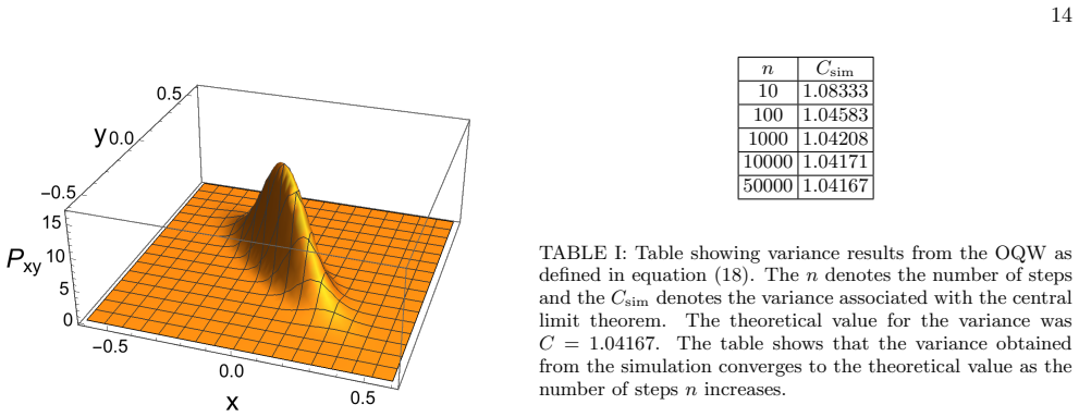
Take the lazy open quantum walk of the numerical example, where the theoretical variance is $C = 1.04167$, simulate a large number of independent trajectories, and test the empirical rescaled positions $(X_n - n m)/\sqrt{n}$ against the Gaussian $N(0,C)$ with a standard goodness-of-fit test; a discrepancy that does not shrink as $n$ grows would refute the theorem. A complementary check is to build a homogeneous lazy walk whose operator algebra decouples into two sectors, each with its own steady state, and verify that the rescaled position fails to converge to a single Gaussian, confirming that the uniqueness assumption is essential.

Watch

Extended reading notes

Core claim

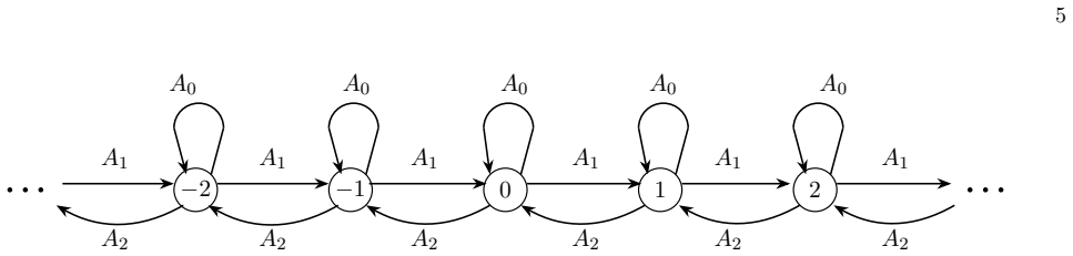
The central claim is that a homogeneous lazy open quantum walk on $\mathbb{Z}^d$, whenever the completely positive map $L(\tau)=\sum_{j=0}^{2d} A_j \tau A_j^\dagger$ has a unique steady state $\rho_\infty$, satisfies $(X_n - n m)/\sqrt{n}$ converging in distribution to a centered Gaussian with covariance $C$, where $m$ is the mean jump vector and $C$ is the explicit expression in formula (35). The proof passes to the quantum-trajectory picture, where the walk becomes a classical Markov chain, and decomposes the position process into a martingale plus a bounded predictable part. Verifying the two martingale central limit theorem conditions, with the quadratic variation controlled by the ergodic theorem for the unique steady state, yields the Gaussian law. Because the lazy operator $A_0$ enters both the map and its dual, the steady state $\rho_\infty$, the mean $m$, and the $L_i$ operators defined by $L_i - L^\dagger(L_i) = \tilde A_i - m_i I$ all differ from their non-lazy counterparts, so formula (35) genuinely describes the lazy model. A key added observation is that the system of equations for the $L_i$ is degenerate, with solutions unique up to a multiple of the identity.

Load-bearing premise

The entire result rests on the assumption that the map $L(\tau)=\sum_{j=0}^{2d} A_j \tau A_j^\dagger$ has exactly one steady state $\rho_\infty$; if several steady states coexist, the ergodic convergence and the covariance formula are not justified, and the authors explicitly note that the theorem may then fail.

Editorial extensions

If this is right

Every open quantum walk that comes from a microscopic derivation includes a self-jump term, so the theorem applies to all such walks on a lattice: their long-time position distribution is Gaussian whenever the steady state is unique.
The covariance matrix of that Gaussian can be computed directly from $\rho_\infty$ and the $L_i$ operators, giving an analytic prediction for the diffusion tensor of a dissipative walker.
Ignoring the self-jump systematically changes the predicted mean and variance, so comparisons to experiment must use the lazy formulas rather than the non-lazy ones.
The degeneracy of the $L_i$ equation, with uniqueness up to a multiple of the identity, simplifies the task of solving for the covariance in real models.
In the microscopic limit, both the steady-state equation and the evolution equation for $L_l$ become independent of the time step and take a standard dissipative master-equation form, connecting the discrete-time theorem to the continuous-time master equation.

Reading between the lines

Editorial extensions of the paper, not claims the author makes directly.

If the uniqueness assumption fails but the steady states form a convex set, a plausible extension is a conditional central limit theorem: the limiting law would be a mixture of Gaussians weighted by the initial state's projection onto each ergodic sector, with the same covariance formula applied sector by sector.
The Fourier-space dual method used for non-lazy open quantum walks could be applied to the lazy map, offering an independent derivation of formula (35) and possibly stronger local limit theorems for these walks.
Because the self-jump probability can be tuned experimentally, formula (35) suggests a direct test in optical-lattice or trapped-ion implementations: vary the lazy operator and compare the measured diffusion constant with the analytic prediction.

Share X Bluesky LinkedIn Reddit HN

Signed reviews

No signed human review yet.

Editorial analysis

A structured set of objections, weighed in public.

Desk editor's note, referee report, and a circularity audit.

Desk Editor's Note

read the letter

Main thing: the paper extends the OQW central limit theorem to lazy walks where a self-loop A0 is allowed, and gives an explicit covariance formula (35). The physical motivation is solid: [40] showed microscopically derived OQWs must have a self-jump term. The explicit treatment of A0 in the variance is not in [28], and the numerical check in Section III.E is genuine and convincing: the simulated variance converges to the predicted value as n grows, with no fitting constants. The connection to the microscopic GKSL form is also useful.

The soft spot is the proof. The martingale CLT is not actually supplied. Condition (33) is fine, but the load-bearing condition (34) is dismissed with "one can show" and a reference to the ergodic theorem (22). The stress-test note is right: Cesaro convergence of tau_n to rho_infinity does not imply convergence of the nonlinear functions in the conditional variance, and the lazy transition kernel differs, so the estimates from [28] do not automatically transfer. I suspect it can be fixed, but as written the central theorem is asserted, not proved. The relation to [35], which already proved a CLT for homogeneous OQWs on Z^d, is also not resolved: if [35] covers arbitrary finite jumps including zero displacement, then the CLT is not new; only the variance formula and the microscopic connection are.

Unique steady state is assumed and flagged, which is fine. The algebraic checks in the microscopic examples are consistent, though they check the variance formula rather than the CLT itself.

Overall: a clearly written, physically motivated paper for the OQW community, but the main theorem is incomplete and novelty relative to [35] is unclear. It deserves a serious referee, not a desk rejection; acceptance should require filling the gap in (34) and clarifying the prior literature.

Referee Report

3 major / 3 minor

Summary. The paper extends the discrete-time open quantum walk by adding a 'lazy' Kraus operator A0 that leaves the lattice site unchanged. For a homogeneous lazy OQW on Z^d with a unique steady state, it claims a central limit theorem: (X_n - n m)/sqrt(n) converges in distribution to a Gaussian, with mean m and covariance matrix C_ij given by Eq. (35). The derivation follows [28]: a Doob decomposition turns the centered position into a martingale plus a bounded term, and a martingale CLT is invoked. The paper also connects the lazy map to a microscopic master equation, supplies analytic variance formulas for one- and two-dimensional microscopic models, and reports a numerical simulation (Table I) confirming the variance formula for a specific one-dimensional walk.

Significance. If the CLT is established, the paper fills a physically motivated gap: [40] showed that any microscopically derived OQW must contain a self-jumping term, so the lazy version is the relevant object for applications. The variance formula (35) is concrete and falsifiable, and the numerical check in Section III E is an independent test with no fitted parameters; the analytic examples in Sections III C and III D also reproduce the microscopic expressions of [40], which supports the internal consistency of the calculation. The main weakness is that the proof of the martingale condition (34) is not supplied, so the central result is currently an assertion rather than a demonstrated theorem; the numerical and analytic checks make the claim plausible but do not replace the missing verification.

major comments (3)

[III A, Eqs. (33)-(34)] Equation (34) is the load-bearing condition for the martingale CLT, but it is not proved. The integrand E[(Delta M_k)^2 | F_{k-1}] is a nonlinear function of tau_{k-1} (it involves p_j = Tr(A_j tau_{k-1} A_j^dag) and the normalized post-jump states A_j tau_{k-1} A_j^dag / p_j). The cited ergodic theorem (22) only asserts almost-sure Cesaro convergence of the internal states tau_j to rho_infty; this alone does not imply convergence of Cesaro averages of nonlinear functions of the full chain (tau_n, Delta X_n) unless an ergodic theorem for that chain is stated and its hypotheses (e.g., irreducibility/aperiodicity or a unique invariant measure for the trajectory chain) are verified. The assertion 'one can show' therefore hides the main step, and formula (35) is not rigorously derived.
[III A, Eqs. (24)-(26)] The statement that the increments Y_k are i.i.d. once the system is in the steady state is not correct for the quantum trajectory chain. Even with the marginal law of tau_n equal to rho_infty, the increment Delta X_n has conditional distribution P(j,n) = Tr(A_j tau_n A_j^dag) that depends on the random internal state tau_n, so successive increments are dependent. The i.i.d. setup in Eqs. (24)-(26) is also inconsistent with the martingale decomposition that follows: if the increments were i.i.d., the covariance in (35) would reduce to sum_j p_j e_j e_j^T - m m^T and the L-dependent terms would be absent. The theorem should be formulated for the stationary Markov chain used in [28].
[III A, Eqs. (28a) and (35)] The Poisson equation (28a) and the covariance formula (35) are taken from [28], but the lazy walk changes both L and L^dag through the extra operator A0. Consequently the existence of L_l and the convergence of the conditional variance are not automatic consequences of the non-lazy theorem; the manuscript must either state the exact theorem from [28] in a form covering the present transition kernel and verify its hypotheses, or give a self-contained proof. The current one-sentence justification of (34) does not do either. Additionally, the uniqueness of the fixed point of L is assumed, but no condition ensuring ergodicity of the trajectory chain is supplied, so uniqueness by itself is not shown to be sufficient.

minor comments (3)

[III A, Eq. (31)] The vectorized left-hand side of Eq. (28a) should be (I - sum_{i=0}^{2d} A_i^dag tensor A_i^T) vec(L_l); the sum as written starts at i=1 and omits A0, although L^dag includes i=0 and the numerical matrix in Eq. (87) includes the A0 contribution.
[II A] The phrase 'l2(C) is the space of square integrable functions' should read 'the space of square-summable sequences on Z^d'; also 'posseses' should be 'possesses'.
[III D, Example 2] In Eqs. (66)-(67), both B_y and C_y are defined with sigma_z, but C_y is later used in the combination r_- = gamma_+^y - gamma_-^y as a backward transition; the relation of these operators to the positive and negative y-directions e_2 and e_4 should be stated explicitly.

Circularity Check

0 steps flagged · score 0.0 of 10

No significant circularity: the CLT covariance is computed from the model's steady state and Poisson-type equation, with independent numerical verification; self-citations are motivational, not load-bearing.

full rationale

The derivation's central output, the covariance formula (35), is not fitted or defined in terms of the predicted distribution: it is obtained by solving the steady-state condition L(rho_infty)=rho_infty and the Poisson-type equation (28a)/(32) for L_i, then evaluating an analytic expression. The mean m is likewise computed from rho_infty and the jump operators. The numerical check in Section III E uses the fixed operators in (18), simulates trajectories, and compares the empirical variance with the value C=1.04167 from formula (35); no parameter is adjusted, so this is an independent check rather than a fitted-input-called-prediction. The martingale framework is cited to [28] (Attal et al.), an external published proof, and the lazy extension consistently replaces L with the map including A0; while the proof of condition (34) is only sketched ('one can show'), that is a rigor gap, not circularity. The self-citation to [40] supports the motivation that microscopically derived OQWs are lazy, but it does not enter the mathematical derivation of the CLT: even if that physical claim were absent, the lazy OQW model and its CLT as stated would stand. No step reduces by construction to its own input.

Assumptions & free parameters 0 free parameters · 4 assumptions · 0 invented entities

The central result rests on standard martingale central limit theory, the existing CLT machinery from [28], and the physical assumption of a unique steady state for the coin. No new physical entities or fitted parameters are introduced.

assumptions (4)

domain assumption The steady state rho_infty of L(tau)=sum_j A_j tau A_j^dagger is unique.
The CLT and covariance formula use the ergodic average (22); without uniqueness, the trajectory may switch between steady states and the variance limit may fail. The paper states this assumption in Section II B and the Conclusion.
domain assumption The quantum trajectory process satisfies the almost-sure ergodic convergence (1/n) sum_tau_t -> rho_infty.
Quoted from [27]; needed to evaluate the conditional variance in the martingale CLT.
domain assumption The martingale CLT conditions (33) and (34) hold for the lazy OQW trajectory.
The paper asserts these conditions with one-line justifications ("it is straightforward" and "one can show") and does not provide a detailed proof.
domain assumption Equation (28a) has a solution L_l for each l, unique up to addition of a multiple of the identity.
This is a theorem from [28] that the paper relies on; the paper shows the system is degenerate but refers to [28] for existence and uniqueness up to identity.

how reviews work

0 comments

Cite this review

Pith. "Pith review of Lazy Open Quantum Walks." pith.science (2026). https://pith.science/paper/MU4XV5YF

@misc{pith2026190804124,
  author       = {Pith},
  title        = {Pith review of: Lazy Open Quantum Walks},
  year         = {2026},
  howpublished = {\url{https://pith.science/paper/MU4XV5YF}},
  note         = {Machine review of arXiv:1908.04124}
}

abstract

Open quantum walks (OQWs) describe a quantum walker on an underlying graph whose dynamics is purely driven by dissipation and decoherence. Mathematically, they are formulated as completely positive trace preserving (CPTP) maps on the space of density matrices for the walker on the graph. Any microscopically derived OQW must include the possibility of remaining on the same site on the graph when the map is applied. We extend the CPTP map to describe a lazy OQW. We derive a central limit theorem for lazy OQWs on a $d$-dimensional lattice, where the distribution converges to a Gaussian. We show that the properties of this Gaussian computed using conventional methods agree with the general formulas derived from our central limit theorem.

Figures

Figures reproduced from arXiv: 1908.04124 by the authors.

**Figure 2.** FIG. 2: The above figure is an illustration of the homogeneous [PITH_FULL_IMAGE:figures/full_fig_p004_2.png] view at source ↗

**Figure 3.** FIG. 3: This figure depicts the discrete homogeneous lazy OQW on the line. The operators [PITH_FULL_IMAGE:figures/full_fig_p005_3.png] view at source ↗

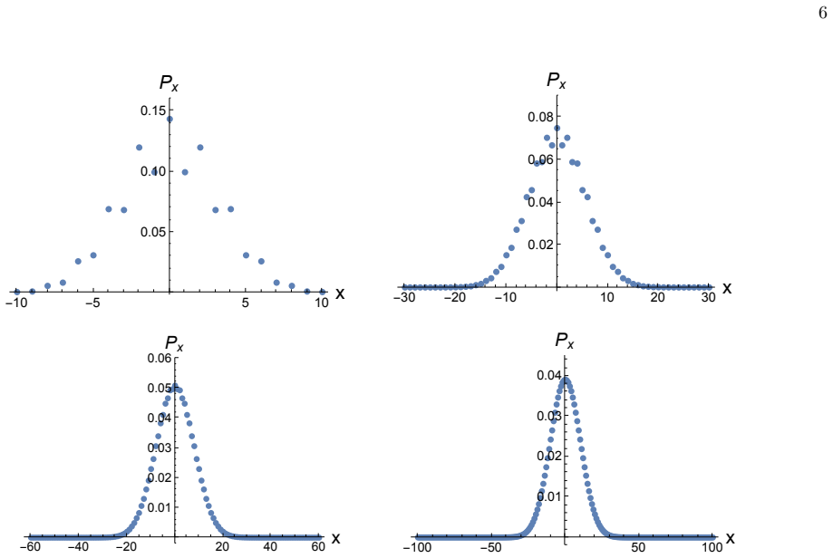
Figures from the paper (4 more)

**Figure 4.** Figure 4: FIG. 4: In these four figures, we ran the OQW for the operators defined in equation (18) for 10 [PITH_FULL_IMAGE:figures/full_fig_p006_4.png]

**Figure 5.** Figure 5: FIG. 5: The Gaussian distribution plotted from the theo [PITH_FULL_IMAGE:figures/full_fig_p011_5.png]

**Figure 6.** Figure 6: FIG. 6: The Gaussian distribution plotted from the theoreti [PITH_FULL_IMAGE:figures/full_fig_p013_6.png]

**Figure 7.** Figure 7: FIG. 7: The Gaussian distribution plotted from the theo [PITH_FULL_IMAGE:figures/full_fig_p014_7.png]

Discussion (0). Continue with ORCID to comment.

Reference graph

Works this paper leans on

56 extracted references · 48 canonical work pages

[35]

Attal, N

S. Attal, N. Guillotin-Plantard, and C. Sabot, Ann. Henri Poincare 16 (2012)

work page 2012
[40]

Sinayskiy and F

I. Sinayskiy and F. Petruccione, Physica Scripta 2012, 014077 (2012)

work page 2012
[28]

T. G. Wong, Quantum Information Processing 17 (2018), ISSN 1573-1332

work page 2018
[1]

(22) We further assume that the steady state ρ∞ is unique

For quantum trajectories in discrete time, the sequence 1 n n∑ t=1 τt converges almost surely to a random steady state ρ∞ [27]: 1 n n∑ j=1 τj a.s −→ρ∞. (22) We further assume that the steady state ρ∞ is unique. The central limit theorem formulated in the follow- ing section will be formulated in terms of the ran- dom variables (τn, ∆Xn), where ∆Xn = Xn−Xn...

work page
[2]

To end up with OQW on 2 D one needs to assumes an environment assisted transport between every connected node of the walk

Example 2 Let us consider 2D array of two level atoms (for ex- ample, trapped ultra cold atoms on an optical lattice) 12 described by the following Hamiltonian: HS = ∑ r ω0 2 σz⊗|r⟩⟨r| +λ (⃗ nλ⃗ σ)⊗|r⟩⟨r|, (63) where σz is Pauli z matrix and describes internal degree of freedom of the walker and |r⟩≡| i,j⟩ describes posi- tion of the on 2 D lattice. To en...

work page
[3]

In both examples, the transition oper- ators will follow from the outlined microscopic model for lazy OQWs in 2 D

Generic notations In this subsection two examples of lazy OQWs in 2 D will be presented. In both examples, the transition oper- ators will follow from the outlined microscopic model for lazy OQWs in 2 D. To make notations more clear, the following conventions will be used: • coordinates on the 2D lattice r = (i,j ); • possible movement from the r along th...

work page
[4]

C. H. Papadimitriou, Computational Complexity (Addison-Wesley, Reading, MA, 1994)

work page 1994
[5]

From the microscopic point of view, this means that the only diﬀerence to the previous example would be in the form of the interaction Hamiltonian

Example 3 In this example, it is assumed that the transition of the walker along both axes is assisted via a dissipative coupling. From the microscopic point of view, this means that the only diﬀerence to the previous example would be in the form of the interaction Hamiltonian. Under these assumptions, the system-bath Hamiltonian HSB is 13 FIG. 6: The Gau...

work page

Show all 56 references

[6]

2 [ − 2⟨n⟩rs2 2γ2 x ( 4λ2 + (⟨n⟩ + 1)r2s2 ) + 8λ2rγ2 x ( −4λ2(4⟨n⟩(⟨n⟩ + 2) + 3)−⟨n⟩r2s3 2 ) 8λ2 +r2s2 2 +s1γx ( 8λ2 +r2s2 2 )( 4λ2 +⟨n⟩r2s2 ) +⟨n⟩γx ( 4λ2 +r2s1s2 )( 8λ2 +r2s2 2 )] (81) Cxy = −2∆γxγy ( 8λ4( 8⟨n⟩2 + 8⟨n⟩ + 6 ) rs2 +⟨n⟩r5s1s5 2 + 16λ2⟨n⟩r3s1s3 2 ) (8λ2 +r2s2
[7]

(82) In (81),r =γx +γy

3 . (82) In (81),r =γx +γy. Cyy is the same expression but with γx and γy interchanged. We found the oﬀ-diagonal ele- ments to be given by (82). We note that Cyx =Cxy and that the oﬀ-diagonal elements are symmetric under in- terchangingγx andγy. Figure 7 shows the Gaussian dis...
[8]

Barber, N

M. Barber, N. Nakanishi, B. Ninham, and B. Ninham, Random and Restricted Walks: Theory and Applications , Mathematics and its applications : a series of mono- graphs and texts (Gordon and Breach, 1970)

1970
[9]

F. B. Knight, Transactions of the American Mathemati- cal Society 103, 218 (1962)

1962
[10]

G. H. Weiss and R. J. Rubin, Adv. Chem. Phys. 52, 363 (2007)

2007
[11]

Konno, Journal of the Mathematical Society of Japan 57, 1179 (2005)

N. Konno, Journal of the Mathematical Society of Japan 57, 1179 (2005)

2005
[12]

Cootner, The random character of stock market prices (M.I.T

P. Cootner, The random character of stock market prices (M.I.T. Press, 1964)

1964
[13]

Berg, Random Walks in Biology , Princeton paper- backs (Princeton University Press, 1993)

H. Berg, Random Walks in Biology , Princeton paper- backs (Princeton University Press, 1993)

1993
[14]

Aharonov, L

Y. Aharonov, L. Davidovich, and N. Zagury, Phys. Rev. A 48, 1687 (1993)

1993
[15]

Farhi and S

E. Farhi and S. Gutmann, Phys. Rev. A 58, 915 (1998)

1998
[16]

Kempe, Contemporary Physics 44, 307 (2003)

J. Kempe, Contemporary Physics 44, 307 (2003)

2003
[17]

S. E. Venegas-Andraca, Quant. Inf. Proc. 11, 1015 (2012), 1201.4780

2012 arXiv
[18]

L. Dan, M. M. Gettrick, Z. Wei-Wei, and Z. Ke-Jia, Chi- nese Physics B 24, 050305 (2015)

2015
[19]

Reitzner, D

D. Reitzner, D. Nagaj, and V. Buˇ zek, Acta Physica Slo- vaca 61, 603 (2011)

2011
[20]

A. M. Childs, Communications in Mathematical Physics 294, 581 (2010)

2010
[21]

L. K. Grover, in Proceedings of the Twenty-Eighth Annual ACM Symposium on Theory of Computing (Association for Computing Machinery, New York, NY, USA, 1996), STOC ?96, p. 212?219, ISBN 0897917855

1996
[22]

T. G. Wong, Journal of Physics A Mathematical General 48, 435304 (2015), 1502.04567

2015 arXiv
[23]

N. Inui, N. Konno, and E. Segawa, Phys. Rev. E 72, 056112 (2005)

2005
[24]

ˇStefaˇ n´ ak, I

M. ˇStefaˇ n´ ak, I. Bezdˇ ekov´ a, and I. Jex, Phys. Rev. A90, 012342 (2014)

2014
[25]

Petruccione and I

F. Petruccione and I. Sinayskiy, Phys. Scr. T151, 014077 (2012)

2012
[26]

M. L. Rhodes and T. G. Wong, Phys. Rev. A100, 042303 (2019)

2019
[27]

P. R. Giri and V. Korepin, Modern Physics Letters A p. 2050043 (2019), ISSN 1793-6632

2019
[29]

Q.-P. Su, Y. Zhang, L. Yu, J.-Q. Zhou, J.-S. Jin, X.-Q. Xu, S.-J. Xiong, Q. Xu, Z. Sun, K. Chen, et al., npj Quantum Information 5, 40 (2019), 1805.09784

2019 arXiv
[30]

Attal, F

S. Attal, F. Petruccione, C. Sabot, and I. Sinayskiy, J. Stat. Phys. 147, 832 (2012)

2012
[31]

Attal, F

S. Attal, F. Petruccione, and I. Sinayskiy, Physics Letters A 376, 1545 (2012), ISSN 0375-9601

2012
[32]

Sadowski and L

P. Sadowski and L. Pawela, Quantum Information Pro- cessing 15, 2725 (2016)

2016
[33]

Sinayskiy and F

I. Sinayskiy and F. Petruccione, Quantum Information Processing 11, 1301 (2012)

2012
[34]

Kummerer and H

B. Kummerer and H. Maassen, Journal of Physics A: Mathematical and General 37, 11889 (2004)

2004
[36]

Konno and H

N. Konno and H. J. Yoo, Journal of Statistical Physics 150, 299 (2013), 1209.1419

2013 arXiv
[37]

Pellegrini, Journal of Statistical Physics 154, 838 (2014)

C. Pellegrini, Journal of Statistical Physics 154, 838 (2014)

2014
[38]

Bringuier, Annales Henri Poincar´ e18, 3167 (2017)

H. Bringuier, Annales Henri Poincar´ e18, 3167 (2017)

2017
[39]

Sinayskiy and F

I. Sinayskiy and F. Petruccione, The European Physical Journal Special Topics 227, 1869 (2019)

2019
[41]

Carbone and Y

R. Carbone and Y. Pautrat, Annales Henri Poincar´ e17, 99 (2016)

2016
[42]

Carbone and Y

R. Carbone and Y. Pautrat, Journal of Statistical Physics 160, 1125 (2015)

2015
[43]

C. F. Lardizabal and R. R. Souza, Journal of Statistical Physics 164, 1122 (2016)

2016
[44]

Bauer, D

M. Bauer, D. Bernard, and A. Tilloy, Phys. Rev. A 88, 062340 (2013)

2013
[45]

Bauer, D

M. Bauer, D. Bernard, and A. Tilloy, Journal of Statis- tical Mechanics: Theory and Experiment 2014, P09001 (2014)

2014
[46]

The Hamiltonian for the total system may be written as the sum of the system, bath and system-bath interactions Hamiltonians, H =HS +HB +HSB

culminating in [40]. The Hamiltonian for the total system may be written as the sum of the system, bath and system-bath interactions Hamiltonians, H =HS +HB +HSB. (37) The system Hamiltonian describes the local free evolu- tion of the walker’s internal degree of freedom as wel...
[47]

Sinayskiy and F

I. Sinayskiy and F. Petruccione, Phys. Rev. A 92, 032105 (2015)

2015
[48]

Kraus, A

K. Kraus, A. B¨ ohm, J. D. Dollard, and W. H. Wootters, States, Eﬀects, and Operations Fundamental Notions of Quantum Theory, vol. 190 (1983)

1983
[49]

Doob, Stochastic Processes , Wiley Publications in Statistics (John Wiley & Sons, 1953), ISBN 9780471218135

J. Doob, Stochastic Processes , Wiley Publications in Statistics (John Wiley & Sons, 1953), ISBN 9780471218135

1953
[50]

Hall and C

P. Hall and C. Heyde, Martingale limit theory and its ap- plication, Probability and mathematical statistics (Aca- demic Press, 1980)

1980
[51]

Williams, Probability with Martingales , Cambridge mathematical textbooks (Cambridge University Press, 1991)

D. Williams, Probability with Martingales , Cambridge mathematical textbooks (Cambridge University Press, 1991)

1991
[52]

W. F. Stinespring, Proceedings of the American Mathe- matical Society 6, 211 (1955)

1955
[53]

Sinayskiy and F

I. Sinayskiy and F. Petruccione, International Journal of Quantum Information 12, 1461010 (2014)

2014
[54]

Breuer and F

H. Breuer and F. Petruccione, The Theory of Open Quan- 16 tum Systems (OUP Oxford, 2007)

2007
[55]

Gorini, A

V. Gorini, A. Kossakowski, and E. C. G. Sudarshan, Journal of Mathematical Physics 17, 821 (1976)

1976
[56]

Lindblad, Communications in Mathematical Physics 48, 119 (1976)

G. Lindblad, Communications in Mathematical Physics 48, 119 (1976)

1976

Pith tools

Reviewed August 14, 2026 · model on record in the stance chip above.

[1] [35]

Attal, N

S. Attal, N. Guillotin-Plantard, and C. Sabot, Ann. Henri Poincare 16 (2012)

work page 2012

[2] [40]

Sinayskiy and F

I. Sinayskiy and F. Petruccione, Physica Scripta 2012, 014077 (2012)

work page 2012

[3] [28]

T. G. Wong, Quantum Information Processing 17 (2018), ISSN 1573-1332

work page 2018

[4] [1]

(22) We further assume that the steady state ρ∞ is unique

For quantum trajectories in discrete time, the sequence 1 n n∑ t=1 τt converges almost surely to a random steady state ρ∞ [27]: 1 n n∑ j=1 τj a.s −→ρ∞. (22) We further assume that the steady state ρ∞ is unique. The central limit theorem formulated in the follow- ing section will be formulated in terms of the ran- dom variables (τn, ∆Xn), where ∆Xn = Xn−Xn...

work page

[5] [2]

To end up with OQW on 2 D one needs to assumes an environment assisted transport between every connected node of the walk

Example 2 Let us consider 2D array of two level atoms (for ex- ample, trapped ultra cold atoms on an optical lattice) 12 described by the following Hamiltonian: HS = ∑ r ω0 2 σz⊗|r⟩⟨r| +λ (⃗ nλ⃗ σ)⊗|r⟩⟨r|, (63) where σz is Pauli z matrix and describes internal degree of freedom of the walker and |r⟩≡| i,j⟩ describes posi- tion of the on 2 D lattice. To en...

work page

[6] [3]

In both examples, the transition oper- ators will follow from the outlined microscopic model for lazy OQWs in 2 D

Generic notations In this subsection two examples of lazy OQWs in 2 D will be presented. In both examples, the transition oper- ators will follow from the outlined microscopic model for lazy OQWs in 2 D. To make notations more clear, the following conventions will be used: • coordinates on the 2D lattice r = (i,j ); • possible movement from the r along th...

work page

[7] [4]

C. H. Papadimitriou, Computational Complexity (Addison-Wesley, Reading, MA, 1994)

work page 1994

[8] [5]

From the microscopic point of view, this means that the only diﬀerence to the previous example would be in the form of the interaction Hamiltonian

Example 3 In this example, it is assumed that the transition of the walker along both axes is assisted via a dissipative coupling. From the microscopic point of view, this means that the only diﬀerence to the previous example would be in the form of the interaction Hamiltonian. Under these assumptions, the system-bath Hamiltonian HSB is 13 FIG. 6: The Gau...

work page