REVIEW 3 minor 58 references
Design-Based Prediction-Powered Inference for Spatial Data
T0 review · 0 major / 3 minor · reviewed 2026-08-15 · deepseek-v4-flash
Pith's one-line read Double robustness breaks for spatial PPI when the propensity is wrong
desk verdict Worth a serious referee: the genuinely new result is Theorem 1's exact finite-population gap identity under spatial residuals; the rest is a transparent, useful translation of survey sampling into PPI, with the ratio-stable labelling caveat properly flagged. read the letter →
The pith
A machine-rendered reading of the paper's core claim, the machinery that carries it, and where it could break.
The reading
What carries the argument
The central object is the gap identity of Theorem 1, built from the weight-ratio field $v_i = \pi_i/\tilde\pi_i - \overline{\pi/\tilde\pi}$ and the residual correlation matrix $P=[\rho_u(s_i,s_j)]$. The effective sample size $N_{\mathrm{eff},v} = (N\bar h)^2/(v^\top P v)$ counts how many independent patches of residual error the misspecified weights actually see; it is $O(N)$ for i.i.d. or exchangeable residuals and can be $O(1)$ under spatially coherent dependence. This identity carries the argument because it shows that the conditional finite-population remainder is free of the label count under ratio-stable labelling, and that correcting the propensity (making $v\equiv 0$) kills it while correcting the outcome model does not.
What would settle it
Enumerate a fixed spatial population with known outcomes and map, draw many label sets at several budgets under a deliberately misspecified propensity plus a correct outcome model, and track the conditional bias and coverage of the self-normalised AIPW estimator on the same population. Theorem 1 predicts the bias stays constant at $G_U$ and coverage falls once $\sqrt{n}|G_U|$ grows; observing the bias shrink with $n$ or coverage recover would refute it.
Extended reading notes
Core claim
The paper's central claim is Theorem 1: in a fixed spatial population, with the outcome model correctly specified and the propensity model misspecified, the self-normalised doubly robust PPI estimator decomposes as design error $O_p(n^{-1/2})$ plus a conditional gap $G_U = (N\bar h)^{-1}\sum_{i\in U} v_i u_i$, where $h_i = \pi_i/\tilde\pi_i$ is the ratio of true to pseudo-true inclusion probability, $v_i = h_i - \bar h$, and $u_i$ is the outcome-model residual. Conditionally on the realised population, $G_U$ is a fixed number, its superpopulation variance is $\sigma_u^2 / N_{\mathrm{eff},v}$ with $N_{\mathrm{eff},v} = (N\bar h)^2/(v^\top P v)$, and under ratio-stable labelling it does not depend on $n$. Consequently, as labels accumulate, the fixed gap is divided by a shrinking design standard error and coverage can fall; a correct propensity sets $v=0$ and removes the gap, whereas spatial correlation of $u$ can inflate $v^\top P v$ and shrink the effective patch count.
Load-bearing premise
The key assumption is that the map-error field has zero mean under the working model and that the misspecified selection weights vary in step with that field's spatial correlation; if either fails, the non-shrinking gap disappears or changes size.
Editorial extensions
If this is right
- For a fixed spatial population under simple random sampling, spatial correlation of the map error never enters the design variance, so i.i.d.-style PPI intervals hold nominal coverage and the map only shortens the interval.
- Under clustered labelling, using the i.i.d. variance formula can lower coverage to 58% as the error field becomes smooth; a cluster-robust variance is required.
- Spatially balanced one-per-block sampling reduces the design variance exactly when between-block variation exceeds $(n-1)/(N-n)$ times the average within-block variation; below that threshold it buys nothing.
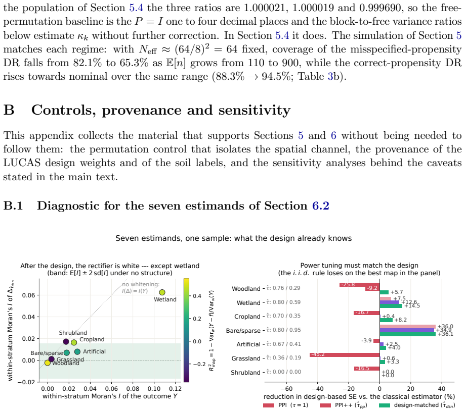
- The design-matched power-tuning coefficient, which minimises the stratified design variance, differs from the pooled PPI++ coefficient whenever the design has already removed between-stratum covariance, and using the pooled value can lose precision on the best maps.
- With a misspecified propensity and a correct outcome model, the doubly robust estimator's conditional bias is the fixed gap $G_U$; coverage erodes once the design standard error falls below $|G_U|$, so enlarging the label budget can make matters worse.
Reading between the lines
- If Theorem 1 transfers to small-area estimation, the exposure is worst where labels are few: borrowing strength across areas reduces sampling variance without touching the propensity misspecification, so the fixed gap becomes relatively larger; the paper names small-area estimation as a likely site but does not formalise it.
- The paper's warning about pooled residual diagnostics suggests a general caution: any Moran-type gate for choosing a spatial variance estimator should be run on design-centred residuals, since a pooled test can flag stratum effects as spatial dependence.
- A testable extension would derive the effective patch count for spatially balanced designs with $\pi_{ij}=0$ on within-block pairs, because Theorem 1's exact identity is stated for independent Bernoulli selection and such designs may change how the gap is evaluated.
Signed reviews
Editorial analysis
A structured set of objections, weighed in public.
Referee Report
Summary. The paper recasts prediction-powered inference (PPI) in a design-based finite-population framework for spatial data. The estimand is a census parameter of a fixed pixel population, with randomness coming only from the labelling mechanism. Sections 3 and 4 provide exact design variances, a threshold for when spatial balance pays, optimal allocation, design-matched power tuning, and sandwich inference for estimated propensities. The main theoretical result, Theorem 1, derives an exact conditional finite-population remainder G_U for doubly robust estimation under a misspecified propensity and a correct outcome model, with variance σ_u^2 / N_eff,v, where N_eff,v is defined by the residual correlation matrix and the weight-ratio field. Under ratio-stable labelling (A8) this remainder does not shrink with the label count, so coverage can deteriorate as n grows when spatial dependence aligns with the weight-ratio field; for i.i.d. or exchangeable residual fields it is negligible when n/N→0. The paper validates the mechanism on a fully enumerated Estonian population of 48,175 cells with only the labelling simulated, and reports Estonian LUCAS land-cover and soil-carbon applications, including an explicit reappraisal of an earlier empirical claim.
Significance. Theorem 1's exact variance identity (9) is a clean and non-circular calculation from the stated model, and the definition of N_eff,v as a variance ratio is substantive rather than tautological: the paper shows that spatial coherence can make N_eff,v of order one, in which case the double-robustness remainder binds at ordinary label counts. This is a genuinely new point at the intersection of PPI and survey sampling. The paper is also unusually careful about its own limitations: Remark 7 notes that the gap is not identified from labels alone under a misspecified propensity, Appendix A.6 discloses the nuisance-rate condition (19) needed when the outcome model is fitted, and Section 7 explicitly narrows the empirical lessons after the soil-carbon study. The semi-synthetic validation on a real fully enumerated population with the labelling simulated, and the scrambling control that isolates the spatial contribution, are strong confirmatory evidence. The reproducible code and the detailed provenance table for each classical result further support the paper's reliability.
minor comments (3)
- [Section 5.3 / Assumption (A8)] The coverage-erosion phenomenon is demonstrated only under the ratio-stable labelling growth of (A8); a brief passage in Section 7 stating that under other growth mechanisms (for example, a fixed-intercept logistic design or simple random sampling with n increasing toward a census) the weight-ratio field v and hence G_U can change with n, so that the erosion is a regime-specific warning rather than a universal law, would help calibrate the practical reading of the abstract.
- [Section 2.3] The double use of h as a stratum subscript and as the weight ratio in Theorem 1 is flagged in the text, but the proximity of objects such as \bar f_{S,h} and h_i in consecutive sections is still easy to misread; adding a one-line cross-reference at the first occurrence of h_i in Section 4 would reduce the notational burden.
- [Section 6.3] In the soil-carbon section, the heading "The corrected claim" could be read as an erratum; renaming it "Refined claim" or "What the diagnostic should read" would better reflect that the authors are generalising a claim rather than retracting it.
Circularity Check
No significant circularity: the central variance identity is a direct calculation from the stated assumptions, and fitted quantities are either explicitly acknowledged as such or checked against an independently enumerated population.
full rationale
The paper's derivation chain is self-contained and does not reduce to its own inputs. Propositions 1-5 are explicitly labeled as translations of standard survey-sampling results, with provenance annotated in Table 7, so their use of external classical results is not circular and no load-bearing self-citation appears. Theorem 1 is a direct calculation: G_U is defined as (N hbar)^{-1} sum_i v_i u_i, and Var_xi(G_U) = sigma_u^2 / N_eff,v with N_eff,v := (N hbar)^2/(v^T P v) is exact algebra from Assumptions (A7) and (A8). The claim that G_U is free of n under ratio-stable labelling is a stated assumption (A8), not a conclusion smuggled in, and the asymptotic classification under i.i.d. or exchangeable fields follows by direct spectral evaluation of v^T P v, not by assuming the answer. The empirical validation in Section 5.3 uses an externally enumerated 48,175-cell population, computes G_U from known propensity ratios and residuals, and then checks that Monte-Carlo bias recovers the precomputed constant; the permutation surrogate for N_eff,v is explicitly described as a surrogate rather than as the exact identity, so no fitted constant is recycled as a prediction. The design-matched power tuning of Proposition 4 is also handled non-circularly: the paper explicitly warns that the clipped optimization cannot lose to the classical estimator by construction and disclaims that as evidence, leaving the empirical content to the size of the gain relative to PPI++. The skeptic's concern about ratio-stable labelling is a robustness or scope limitation about alternative ways to grow n, not a circularity, because the theorem is conditional on the stated growth mechanism and the paper does not claim otherwise. Overall, the derivation is transparent about what is assumed, what is classical, and what is newly calculated.
Assumptions & free parameters
assumptions (9)
- standard math Nested finite-population asymptotics (Isaki and Fuller, 1982) with moment stability (A1).
- domain assumption Design CLT conditions (A3): Hajek-Lindeberg for SRS, rejective and high-entropy designs; for balanced and pivotal designs the paper verifies no design-specific limit conditions.
- domain assumption Relative positivity of true and working propensities (A2)/(A4): c0 n/N <= pi_i <= c1 n/N with no absolute floor.
- domain assumption Correct specification of the logistic propensity in Proposition 5, and pseudo-true propensity with relative positivity in Theorem 1 (A8).
- domain assumption Outcome model is correct: E_xi[u|x] = 0 for residual u = Delta - m(x), with variance sigma_u^2 and correlation matrix P (A7).
- ad hoc to paper Alignment condition lim inf v^T P v / ((N hbar)^2 rbar_U) > 0 and ratio-stability of h (A8).
- ad hoc to paper Anti-concentration of G_U at the origin, uniform over the population sequence (A9).
- ad hoc to paper For Corollary 1, uniform convergence of the empirical Jacobian and diverging componentwise effective sample sizes (A10), especially conditions (12) and (13).
- domain assumption For the empirical LUCAS and soil-carbon illustrations, reconstructed post-stratification weights are treated as inclusion probabilities and the soil-module selection is treated as ignorable within reconstructed strata.
Cite this review
Pith. "Pith review of Design-Based Prediction-Powered Inference for Spatial Data." pith.science (2026). https://pith.science/paper/N2VRFISR
@misc{pith2026260810356,
  author       = {Pith},
  title        = {Pith review of: Design-Based Prediction-Powered Inference for Spatial Data},
  year         = {2026},
  howpublished = {\url{https://pith.science/paper/N2VRFISR}},
  note         = {Machine review of arXiv:2608.10356}
}
abstract
Prediction-powered inference (PPI) combines a wall-to-wall prediction map with a small gold-standard sample to give confidence intervals valid whatever the map's quality. Canonical PPI theory starts from i.i.d.\ labelling, whereas spatial labels arrive through survey designs or covariate-driven mechanisms, and map errors may be spatially correlated. We recast PPI in a design-based framework: the estimand is a census parameter of a fixed spatial population, with randomness arising from the labelling mechanism. We derive exact design variances under simple and stratified sampling, a threshold for when blocked spatial balance pays, and sandwich inference for estimated propensities when selection depends on the map. Our main result concerns double robustness. With a misspecified propensity, a correct outcome model secures superpopulation identification but, conditional on the realised population, leaves a remainder of order $\sigma_u/\sqrt{N_{\mathrm{eff},v}}$, an effective count of the residual patches the weights see. Under ratio-stable labelling this remainder is free of the label count, so coverage can deteriorate as labels accumulate. For i.i.d.\ or exchangeable residual fields $N_{\mathrm{eff},v}$ is of order $N$ and the remainder is negligible beside sampling error when $n/N \to 0$; spatially coherent dependence instead makes it bind. We reproduce this on a fully enumerated population of $48{,}175$ cells. Estonian LUCAS applications show that power tuning and dependence diagnostics must respect the design: i.i.d.\ PPI++ tuning worsens precision for the best map, whereas design-matched tuning cuts standard errors by about $10\%$ and matches or beats PPI++ across seven land-cover estimands. Pooled residual diagnostics can likewise mistake spatially structured between-stratum variation for residual dependence.
Figures


Figures from the paper (6 more)


Reference graph
Works this paper leans on
-
[1]
N., Bates, S., Fannjiang, C., Jordan, M
Angelopoulos, A. N., Bates, S., Fannjiang, C., Jordan, M. I., and Zrnic, T. (2023a). Prediction-powered inference. Science , 382(6671):669--674
work page 2023
-
[2]
Angelopoulos, A. N., Duchi, J. C., and Zrnic, T. (2023b). PPI++ : Efficient prediction-powered inference. arXiv:2311.01453
arXiv 2023
-
[3]
Babcock, C., Finley, A. O., Gregoire, T. G., and Andersen, H.-E. (2018). Remote sensing to reduce the effects of spatial autocorrelation on design-based inference for forest inventory using systematic samples. arXiv:1810.08588
work page Pith review arXiv 2018
-
[4]
Berger, Y. G. (1998a). Rate of convergence for asymptotic variance of the Horvitz--Thompson estimator. Journal of Statistical Planning and Inference , 74(1):149--168
work page 1998
-
[5]
Berger, Y. G. (1998b). Rate of convergence to normal distribution for the Horvitz--Thompson estimator. Journal of Statistical Planning and Inference , 67(2):209--226
work page 1998
-
[6]
Boistard, H., Lopuha \"a , H. P., and Ruiz-Gazen, A. (2017). Functional central limit theorems for single-stage sampling designs. The Annals of Statistics , 45(4):1728--1758
work page 2017
-
[7]
Breidt, F. J. and Opsomer, J. D. (2017). Model-assisted survey estimation with modern prediction techniques. Statistical Science , 32(2):190--205
work page 2017
-
[8]
Brewer, K. R. W. (2002). Combined Survey Sampling Inference: Weighing B asu's Elephants . Arnold, London
work page 2002
Show all 58 references
-
[9]
R., Berlinghieri, R., Bates, S., and Broderick, T
Burt, D. R., Berlinghieri, R., Bates, S., and Broderick, T. (2025). Smooth sailing: Lipschitz -driven uncertainty quantification for spatial associations. In Advances in Neural Information Processing Systems 38 (NeurIPS) . arXiv:2502.06067
2025
-
[10]
M., S \"a rndal, C.-E., and Wretman, J
Cassel, C. M., S \"a rndal, C.-E., and Wretman, J. H. (1976). Some results on generalized difference estimation and generalized regression estimation for finite populations. Biometrika , 63(3):615--620
1976
-
[11]
Chauvet, G. (2012). On a characterization of ordered pivotal sampling. Bernoulli , 18(4):1320--1340
2012
-
[12]
C., and Shi, Z
Chen, S., Chen, Z., Zhang, X., Luo, Z., Schillaci, C., Arrouays, D., Richer-de Forges, A. C., and Shi, Z. (2024). European topsoil bulk density and organic carbon stock database (0--20\,cm) using machine-learning-based pedotransfer functions. Earth System Science Data , 16(5):...
2024 doi
-
[13]
H., Mukherjee, B., and Wu, Z
Chen, X., McCormick, T. H., Mukherjee, B., and Wu, Z. (2025). A unified framework for inference with general missingness patterns and machine learning imputation. arXiv:2508.15162
2025
-
[14]
Chernozhukov, V., Chetverikov, D., Demirer, M., Duflo, E., Hansen, C., Newey, W., and Robins, J. (2018). Double/debiased machine learning for treatment and structural parameters. The Econometrics Journal , 21(1):C1--C68
2018
-
[15]
Conley, T. G. (1999). GMM estimation with cross sectional dependence. Journal of Econometrics , 92(1):1--45
1999
-
[16]
and Caron, F
Cortinovis, S. and Caron, F. (2025). FAB-PPI : Frequentist, assisted by Bayes , prediction-powered inference. In Proceedings of the 42nd International Conference on Machine Learning . arXiv:2502.02363
2025 arXiv
-
[17]
d'Andrimont, R., Yordanov, M., Martinez-Sanchez, L., et al. (2020). Harmonised LUCAS in-situ land cover and use database for field surveys from 2006 to 2018 in the European Union . Scientific Data , 7:352
2020
-
[18]
and Polson, N
Datta, J. and Polson, N. G. (2025). Prediction-powered inference with inverse probability weighting. arXiv:2508.10149 (v2, 2026)
2025
-
[19]
J., Menezes, R., and Su, T.-l
Diggle, P. J., Menezes, R., and Su, T.-l. (2010). Geostatistical inference under preferential sampling. Journal of the Royal Statistical Society: Series C , 59(2):191--232
2010
-
[20]
D'Orazio, M. (2003). Estimating the variance of the sample mean in two-dimensional systematic sampling. Journal of Agricultural, Biological, and Environmental Statistics , 8(3):280--295
2003
-
[21]
M., and Wei, H
Egami, N., Hinck, M., Stewart, B. M., and Wei, H. (2023). Using imperfect surrogates for downstream inference: Design-based supervised learning for social science applications of large language models. In Advances in Neural Information Processing Systems 36 , pages 68589--6860...
2023 arXiv
-
[22]
Emmenegger, N., Stahler, E., and Podimata, C. (2026). Prediction-powered inference across many tasks for AI evaluation and social science research. arXiv:2605.29249
2026 arXiv
-
[23]
A., Dhingra, B., Globerson, A., and Cohen, W
Fisch, A., Maynez, J., Hofer, R. A., Dhingra, B., Globerson, A., and Cohen, W. W. (2024). Stratified prediction-powered inference for hybrid language model evaluation. In Advances in Neural Information Processing Systems 37 . arXiv:2406.04291
2024 arXiv
-
[24]
L., and Datta, A
Gilbert, B., Ogburn, E. L., and Datta, A. (2025). Consistency of common spatial estimators under spatial confounding. Biometrika , 112(2):asae070
2025
-
[25]
o m, A., Lundstr \
Grafstr \"o m, A., Lundstr \"o m, N. L. P., and Schelin, L. (2012). Spatially balanced sampling through the pivotal method. Biometrics , 68(2):514--520
2012
-
[26]
R., Shi, Y., and Cheng, D
Gronsbell, J., Gao, J., McCaw, Z. R., Shi, Y., and Cheng, D. (2024). Another look at statistical inference with machine learning-imputed data. arXiv:2411.19908
2024
-
[27]
H \'a jek, J. (1964). Asymptotic theory of rejective sampling with varying probabilities from a finite population. The Annals of Mathematical Statistics , 35(4):1491--1523
1964
-
[28]
and Eguchi, S
Henmi, M. and Eguchi, S. (2004). A paradox concerning nuisance parameters and projected estimating functions. Biometrika , 91(4):929--941
2004
-
[29]
Hjort, N. L. and Pollard, D. (2011). Asymptotics for minimisers of convex processes. arXiv:1107.3806
2011 arXiv
-
[30]
Isaki, C. T. and Fuller, W. A. (1982). Survey design under the regression superpopulation model. Journal of the American Statistical Association , 77(377):89--96
1982
-
[31]
and Rothenh \"a usler, D
Jin, Y. and Rothenh \"a usler, D. (2024). Tailored inference for finite populations: conditional validity and transfer across distributions. Biometrika , 111(1):215--233
2024
-
[32]
Kilian, V., Cortinovis, S., and Caron, F. (2025). Anytime-valid, Bayes -assisted, prediction-powered inference. In Advances in Neural Information Processing Systems 38 (NeurIPS) . arXiv:2505.18000
2025
-
[33]
Kim, J. K. and Haziza, D. (2014). Doubly robust inference with missing data in survey sampling. Statistica Sinica , 24(1):375--394
2014
-
[34]
M., Lu, K., Zrnic, T., Wang, S., and Bates, S
Kluger, D. M., Lu, K., Zrnic, T., Wang, S., and Bates, S. (2025). Prediction-powered inference with imputed covariates and nonuniform sampling. arXiv:2501.18577
2025
-
[35]
M., Bates, S., and Wang, S
Lu, K., Kluger, D. M., Bates, S., and Wang, S. (2025). Regression coefficient estimation from remote sensing maps. Remote Sensing of Environment , 330:114949. doi:10.1016/j.rse.2025.114949; arXiv:2407.13659
2025
-
[36]
C., and Oberst, M
Mani, P., Xu, P., Lipton, Z. C., and Oberst, M. (2025). No free lunch: Non-asymptotic analysis of prediction-powered inference. arXiv:2505.20178
2025 arXiv
-
[37]
Mat \'e rn, B. (1947). Methods of estimating the accuracy of line and sample plot surveys. Meddelanden fr n Statens Skogsforskningsinstitut , 36(1)
1947
-
[38]
Meng, X.-L. (2018). Statistical paradises and paradoxes in big data (i): law of large populations, big data paradox, and the 2016 us presidential election. The Annals of Applied Statistics , 12(2):685--726
2018
-
[39]
Mozer, R. (2026). PPI is the difference estimator: Recognizing the survey sampling roots of prediction-powered inference. arXiv:2603.19160
2026
-
[40]
M., Herold, M., Stehman, S
Olofsson, P., Foody, G. M., Herold, M., Stehman, S. V., Woodcock, C. E., and Wulder, M. A. (2014). Good practices for estimating area and assessing accuracy of land change. Remote Sensing of Environment , 148:42--57
2014
-
[41]
M., Rotnitzky, A., and Zhao, L
Robins, J. M., Rotnitzky, A., and Zhao, L. P. (1994). Estimation of regression coefficients when some regressors are not always observed. Journal of the American Statistical Association , 89(427):846--866
1994
-
[42]
Salerno, S., Wu, Z., and McCormick, T. H. (2026). Spatially robust inference with predicted and missing at random labels. arXiv:2603.11368
2026
-
[43]
S \"a rndal, C.-E., Swensson, B., and Wretman, J. (1992). Model Assisted Survey Sampling . Springer, New York
1992
-
[44]
M., Parikh, H., and Gu, T
Song, Y., Kluger, D. M., Parikh, H., and Gu, T. (2026). Demystifying Prediction Powered inference. arXiv:2601.20819
2026 arXiv
-
[45]
P., Patterson, P
St hl, G., Saarela, S., Schnell, S., Holm, S., Breidenbach, J., Healey, S. P., Patterson, P. L., Magnussen, S., N sset, E., McRoberts, R. E., and Gregoire, T. G. (2016). Use of models in large-area forest surveys: comparing model-assisted, model-based and hybrid estimation. Fo...
2016
-
[46]
Stevens, D. L. and Olsen, A. R. (2003). Variance estimation for spatially balanced samples of environmental resources. Environmetrics , 14(6):593--610
2003
-
[47]
Stevens, D. L. and Olsen, A. R. (2004). Spatially balanced sampling of natural resources. Journal of the American Statistical Association , 99(465):262--278
2004
-
[48]
and Wilhelm, M
Till \'e , Y. and Wilhelm, M. (2017). Probability sampling designs: principles for choice of design and balancing. Statistical Science , 32(2):176--189. arXiv:1612.04965
2017 arXiv
-
[49]
van der Vaart, A. W. (1998). Asymptotic Statistics . Cambridge University Press
1998
-
[50]
and Esseen, C.-G
von Bahr, B. and Esseen, C.-G. (1965). Inequalities for the r th absolute moment of a sum of random variables, 1 r 2 . The Annals of Mathematical Statistics , 36(1):299--303
1965
-
[51]
Waldetoft, H., Torgander, J., and Magnusson, M. (2025). Prediction-powered estimators for finite population statistics in highly imbalanced textual data: Public hate crime estimation. arXiv:2505.04643
2025 arXiv
-
[52]
Wolter, K. M. (2007). Introduction to Variance Estimation . Springer, New York, 2nd edition
2007
-
[53]
Xu, Z., Witten, D., and Shojaie, A. (2025). A unified framework for semiparametrically efficient semi-supervised learning. arXiv:2502.17741
2025 arXiv
-
[54]
K., and Song, R
Yang, S., Kim, J. K., and Song, R. (2020). Doubly robust inference when combining probability and non-probability samples with high dimensional data. Journal of the Royal Statistical Society: Series B (Statistical Methodology) , 82(2):445--465
2020
-
[55]
Zanaga, D., Van De Kerchove, R., Daems, D., et al. (2022). ESA WorldCover 10\,m 2021 v200. Technical report, European Space Agency. doi:10.5281/zenodo.7254221
2022 doi
-
[56]
Zrnic, T. (2024). A note on the prediction-powered bootstrap. arXiv:2405.18379
2024 arXiv
-
[57]
and Cand \`e s, E
Zrnic, T. and Cand \`e s, E. J. (2024a). Active statistical inference. In Proceedings of the 41st International Conference on Machine Learning , volume 235 of Proceedings of Machine Learning Research . arXiv:2403.03208
2024 arXiv
-
[58]
and Cand \`e s, E
Zrnic, T. and Cand \`e s, E. J. (2024b). Cross-prediction-powered inference. Proceedings of the National Academy of Sciences , 121(15):e2322083121
2024
Reviewed August 15, 2026 · model on record in the stance chip above.
Discussion (0). Continue with ORCID to comment.