REVIEW 2 major objections 4 minor 15 references
Optimal birefringence distributions for star test polarimetry
T0 review · 2 major / 4 minor · reviewed 2026-08-14 · deepseek-v4-flash
Pith's one-line read The paper derives the optimal birefringence distribution for star test polarimetry and shows a stressed-glass optic nearly achieves it.
desk verdict A clean variational derivation showing the stress-engineered glass optic is near-optimal for star test polarimetry; just don't read 'optimal' as a proven global result. read the letter →
The pith
A machine-rendered reading of the paper's core claim, the machinery that carries it, and where it could break.
The reading
What carries the argument
The central object is the Poincaré-sphere/quaternion representation of spatially varying birefringence, $\boldsymbol{\hat{q}}(u)=(q_0,q_1,q_2,q_3)$ with $|\boldsymbol{\hat{q}}|=1$, in which the half-retardance and axis orientation are encoded in the three-vector $\mathbf{q}$. The variational functional $\Delta r^2=\kappa^{-1}\int A^2\|\nabla\boldsymbol{\hat{q}}\|^2d^2u$ ties the PSF broadening directly to the gradient of this unit vector, and the Lagrange-multiplier constraint enforces equal power in the two polarization components. Substitution of the azimuthal ansatz turns the problem into the ordinary differential equation $\bar\delta''(v)+\bar\delta'(v)/v+(\mathrm{NA}^2\Lambda_3 - 1/(2v^2))\sin[2\bar\delta(v)]=0$, whose solution is the fitted quadratic profile. A secondary mechanism is the Fisher information matrix, which converts the PSF shapes into predicted uncertainties in the retrieved Stokes parameters.
What would settle it
Solve the full variational equations, Eqs. (16), without the separable ansatz, allowing arbitrary azimuthal dependence and $q_3\neq0$, and look for a stationary solution with $\langle\boldsymbol{\beta}\rangle_A=0$ and $\Delta r < 0.220\lambda/\mathrm{NA}$; a numerical search that finds any admissible mask with a smaller RMS-width increase would disprove the claimed optimum.
Extended reading notes
Core claim
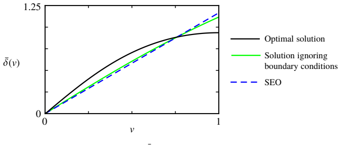
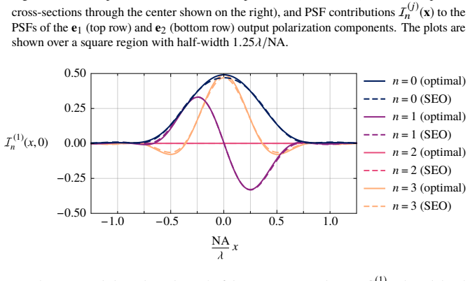
Working in the circular polarization basis and representing the Jones matrix by the unit quaternion $\boldsymbol{\hat{q}}=(q_0,q_1,q_2,q_3)$, the paper derives Euler-Lagrange equations for the birefringence distribution that minimizes $\Delta r^2 = \kappa^{-1}\int A^2 \|\nabla \boldsymbol{\hat{q}}\|^2\,d^2u$ under the equal-power constraint $\langle\boldsymbol{\beta}\rangle_A=0$. For a circular hard aperture, the separable ansatz $\mathbf{q}(u,\phi)=\sin\delta(u)[\cos\phi,\sin\phi,0]$ reduces these equations to a single nonlinear boundary-value problem for the half-retardance $\delta(v)$, Eq. (25), with boundary conditions $\delta(0)=0$ and $\delta'(1)=0$. The numerical solution is essentially quadratic, $\bar\delta(v)\approx 1.856v-0.922v^2$, with an RMS-width increase of $0.220\lambda/\mathrm{NA}$. Compared with the stress-engineered optic's linear profile $\bar\delta(v)=1.166v$, the optimal mask improves FWHM and Strehl by only 5 to 10 percent, and the Fisher-information analysis gives essentially identical expected Stokes-parameter errors, so the conclusion is that the SEO is a near-optimal implementation.
Load-bearing premise
The calculation only searches among masks whose birefringence axis stays in the $q_1q_2$ plane and winds once around the pupil; if the true optimum needs a different axis orientation or a higher-order azimuthal variation, the claimed optimality could fail.
Editorial extensions
If this is right
- A stress-engineered optic with threefold edge stress is, to within 5 to 10 percent in FWHM and Strehl, an optimal birefringence mask for star test polarimetry, so no nanofabricated or programmable mask is needed for near-optimal performance.
- The optimal solution and the SEO both satisfy the equal-power constraint, so the Stokes parameters can be read from a single polarization component's PSF shape without calibrating total power.
- Encoding polarization information costs roughly a 60 percent increase in FWHM and a 50 percent drop in Strehl relative to the diffraction-limited PSF; that is the price of single-shot polarimetry.
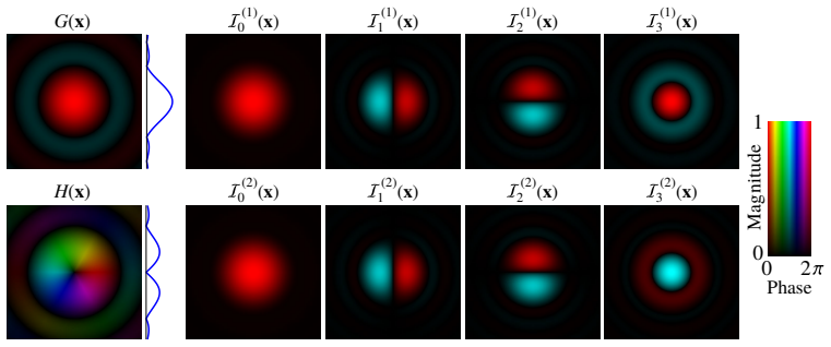
- When both circular components are imaged, the four PSF contributions are nearly orthonormal under the weight $1/I_0^{(1)}(x)$, which simplifies maximum-likelihood retrieval of the Stokes parameters.
- Azimuthal orders $|m|>1$ produce larger PSFs in this framework, so the unit-vortex geometric phase written by the mask is the compact choice for polarization encoding.
Reading between the lines
- If the separable $q_1q_2$ ansatz is relaxed to allow $q_3\ne0$ or non-separable azimuthal dependence, the true optimum could beat $0.220\lambda/\mathrm{NA}$, but the 5 to 10 percent gap to the SEO suggests any further gain would be small.
- The fitted quadratic profile $1.856v-0.922v^2$ could be tested directly by fabricating a mask with that retardance profile and comparing its PSF FWHM to an SEO's; the paper's numbers predict almost no visible difference.
- The same variational machinery could be reapplied to apodized pupils, high-NA vectorial focusing, or other PSF-size metrics; each would shift the optimal $\delta(v)$ slightly, likely preserving the SEO's near-optimality.
Signed reviews
Editorial analysis
A structured set of objections, weighed in public.
Referee Report
Summary. The paper presents a variational calculation to find the birefringence distribution of a pupil-plane mask that minimizes the RMS width increase of the point-spread function (PSF) in star test polarimetry, subject to constraints that ensure equal power in the two circular polarization components and hence a polarization-independent total power. The authors derive the Euler-Lagrange equations (Eqs. 16) and boundary conditions (Eq. 17), first analyze a simplified problem ignoring boundary conditions (Section 6), then propose a separable ansatz q(u,φ)=sinδ(u)[cos(mφ),sin(mφ),0] in Section 7. They solve the resulting nonlinear ODE numerically, find the optimal |m|=1 solution, and give a quadratic approximation δ(v)≈1.856v−0.922v². This solution is compared with the stress-engineered optic (SEO) with δ(v)=1.166v, showing 5–10% differences in FWHM and Strehl ratio. The paper concludes that the SEO is nearly optimal for star test polarimetry and supports this with a Fisher information analysis of measurement accuracy.
Significance. If the optimality claim were fully established, this paper would provide a fundamental benchmark for star test polarimetry and a rigorous explanation of why the simple stress-engineered optic is a near-ideal mask. The work has clear strengths: the variational derivation is careful and internally consistent, the Fisher information analysis is well executed, and the final comparison is quantitative and reproducible from the given equations. The numerical solution is transparent and the approximate fit is useful for practitioners. However, the central claim of global optimality is stronger than what is demonstrated, since the optimization is restricted to a specific symmetric, q3=0 family without proof that the global minimizer lies in this family. This gap affects the title and abstract claims, and also the near-equivalence conclusion for the SEO, which depends on the comparison being made against the true optimum.
major comments (2)
- [Section 7, Eq. (21) and the surrounding text] The global optimality claim is not proven. The paper proposes a separable solution constrained to the q1q2 plane, q(u,φ)=sinδ(u)[cos(mφ),sin(mφ),0], and solves the resulting ODE (Eq. 25) for the half-retardance. This yields a stationary point of the full variational problem only within this restricted family. The objective κ∆r² and the constraints ⟨β⟩=0 are nonconvex (the unit-sphere condition q0²+|q|²=1 is nonlinear), so stationarity within an ansatz does not imply global optimality. A concrete unexplored family is q=sinδ(u)(cosΘ(u)cosφ, cosΘ(u)sinφ, sinΘ(u)), which automatically satisfies ⟨β1⟩=⟨β2⟩=0 and reduces the azimuthal gradient energy by a factor cos²Θ at the cost of additional Θ-gradient terms. Even if the optimal Θ turns out to be zero, that must be demonstrated. As written, the paper establishes at most optimality within the proposed symmetric q3=0 family, and the abstract and title claim 'the optimal birefringence distribution' is therefore too strong. I recommend either providing a symmetry or convexity argument that the global minimizer has this form, or substantially tempering the claims to 'optimal within the proposed family.' Since the SEO near-equivalence conclusion (Table 1) rests on this comparison, the gap is load-bearing.
- [Section 6, text following Eq. (21)] The statement 'there is no loss of generality in this choice, because other solutions can be found through cascading with uniform birefringent plates' is unsupported. Cascading the BM with uniform wave plates can indeed generate other solutions, but it is not shown that every candidate distribution with q3≠0 (or non-separable azimuthal dependence) can be mapped to a q3=0 solution with equal or smaller ∆r while still satisfying the constraints ⟨β⟩=0. The constraints and the RMS width increment are not obviously invariant under such cascading. This matters because the ansatz q3=0 is a key restriction in the derivation of the claimed optimum. The paper should either prove the reduction or explicitly state that q3≠0 distributions are outside the scope of the optimization.
minor comments (4)
- [Section 10, concluding remarks] The phrase 'of a a glass window' contains a duplicated article 'a'.
- [Section 10, concluding remarks] The word 'birefingence' is a typo; it should be 'birefringence'.
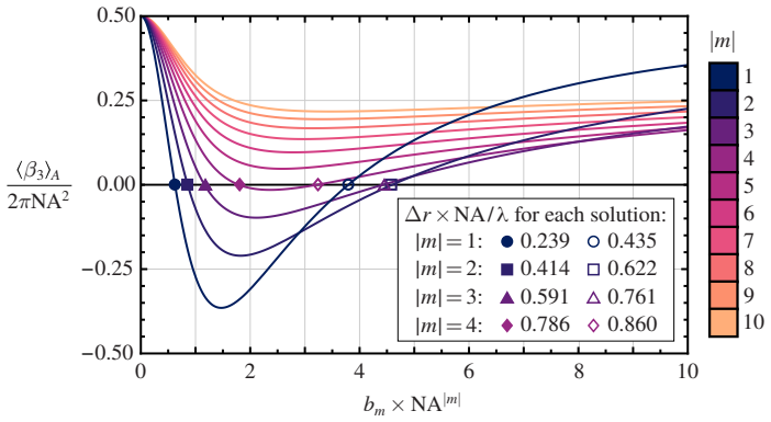
- [Section 8, Eq. (26)] When stating that 'the first one, c = 1.166/NA' is the root that minimizes the width increase, it would be clearer to specify that this is the first nonzero root of Eq. (26), and to note that the root search is over cNA>0.
- [Section 7, Eq. (25) and the fit] The quadratic approximation 1.856v−0.922v² is presented with R²=0.9996, but the paper does not state how the fitting was performed or over what range. Since the numerical solution is already available, the fit is only a presentation aid and could be described as such.
Circularity Check
No circularity: the variational optimum is derived from the defined width metric and constraints, with the SEO appearing only as a comparison benchmark.
full rationale
The paper's central derivation is self-contained: it defines a performance metric (RMS PSF width increase) and constraints (equal power per polarization component), derives the Euler–Lagrange equations from those definitions, and then solves them numerically. The stress-engineered optic is introduced only in Section 8 as a benchmark for comparison, not as an input to the optimization. The separable ansatz in Section 7 (q(u,phi)=sin delta(u)[cos(m phi), sin(m phi), 0]) is an explicit restriction of the search space; it limits the strength of the 'optimal' claim, but it is a stated assumption rather than a circular reduction of the conclusion to the inputs. The quadratic approximation 1.856v - 0.922v^2 is a post-hoc fit to the numerical solution, not a pre-fitted parameter used to produce that solution. Self-citations to Refs. [12], [13], and [15] are for notation, a published mathematical identity, and a tutorial derivation; these either are independently derivable within the paper (the width formula is cross-referenced to the paper's own Eqs. (6) and (7a)) or do not carry the load of the target result. The SEO's c = 1.166/NA is also derived from the equal-power constraint, not fitted to the performance comparison. Thus no circular step is present.
Assumptions & free parameters
free parameters (3)
- b_1 (unconstrained solution amplitude) =
0.625/NA
- SEO stress coefficient c =
1.166/NA
- Shooting parameters for optimal δ (initial slope and NA²Λ3) =
not stated exactly; δ≈1.856v - 0.922v²
assumptions (6)
- standard math Calculus of variations and Fourier optics identities are valid in the paraxial regime.
- domain assumption The imaging system is exit-telecentric with a slow lens, so the paraxial approximation holds and angle-dependent polarization effects at the lens are negligible.
- domain assumption The birefringent mask is thin and described by a Jones matrix of the form in Eq. (1).
- domain assumption RMS irradiance width is an appropriate measure of PSF size, and its near-optimality for other measures is assumed without proof.
- ad hoc to paper The separable ansatz q=sinδ(u)[cos(mφ), sin(mφ),0] contains the global optimum.
- domain assumption Equal power in the two circular components (⟨β⟩A=0) is a necessary constraint for single-image polarimetry.
Cite this review
Pith. "Pith review of Optimal birefringence distributions for star test polarimetry." pith.science (2026). https://pith.science/paper/N7RA6VJZ
@misc{pith2026190802142,
  author       = {Pith},
  title        = {Pith review of: Optimal birefringence distributions for star test polarimetry},
  year         = {2026},
  howpublished = {\url{https://pith.science/paper/N7RA6VJZ}},
  note         = {Machine review of arXiv:1908.02142}
}
read the original abstract
Star test polarimetry is an imaging polarimetry technique in which an element with spatially-varying birefringence is placed in the pupil plane to encode polarization information into the point-spread function (PSF) of an imaging system. In this work, a variational calculation is performed to find the optimal birefringence distribution that effectively encodes polarization information while producing the smallest possible PSF, thus maximizing the resolution for imaging polarimetry. This optimal solution is found to be nearly equivalent to the birefringence distribution that results from a glass window being subjected to three uniformly spaced stress points at its edges, which has been used in previous star test polarimetry setups.
Figures

Figures from the paper (4 more)

Reference graph
Works this paper leans on
-
[12]
Poincaré sphere representation for spatially varying birefringence,
A. Vella and M. A. Alonso, “Poincaré sphere representation for spatially varying birefringence,” Opt. Lett.43, 379–382 (2018)
work page 2018
-
[1]
Band limited data reconstruction in modulated polarimeters,
C. F. LaCasse, R. A. Chipman, and J. S. Tyo, “Band limited data reconstruction in modulated polarimeters,” Opt. Express 19, 14976–14989 (2011)
work page 2011
-
[2]
Stokes-vector and Mueller-matrix polarimetry,
R. Azzam, “Stokes-vector and Mueller-matrix polarimetry,” J. Opt. Soc. Am. A33, 1396–1408 (2016)
work page 2016
-
[3]
Collett, Polarized Light: Fundamentals and Applications (Marcel Dekker, New York, 1993)
E. Collett, Polarized Light: Fundamentals and Applications (Marcel Dekker, New York, 1993)
work page 1993
-
[4]
Single-shot spatially modulated Stokes polarimeter based on a GRIN lens,
J. Chang, N. Zeng, H. He, Y. He, and H. Ma, “Single-shot spatially modulated Stokes polarimeter based on a GRIN lens,” Opt. Lett.39, 2656–2659 (2014)
work page 2014
-
[5]
R. Chipman, “Chapter 22: Polarimetry,” inHandbook of Optics, Vol. II, M. Bass, ed. (McGraw-Hill, New York, 1995)
work page 1995
-
[6]
Star test polarimetry using stress-engineered optical elements,
R. Ramkhalawon, A. M. Beckley, and T. G. Brown, “Star test polarimetry using stress-engineered optical elements,” in Three-Dimensional and Multidimensional Microscopy: Image Acquisition and Processing XIX, vol. 8227 (International Society for Optics and Photonics, 2012), p. 82270Q
work page 2012
-
[7]
Imaging the polarization of a light field,
R. D. Ramkhalawon, T. G. Brown, and M. A. Alonso, “Imaging the polarization of a light field,” Opt. Express21, 4106–4115 (2013)
work page 2013
Show all 15 references
-
[8]
Single-shotpolarimetry imaging of multicore fiber,
S.Sivankutty,E.R.Andresen,G.Bouwmans,T.G.Brown,M.A.Alonso,andH.Rigneault,“Single-shotpolarimetry imaging of multicore fiber,” Opt. Lett.41, 2105–2108 (2016)
2016
-
[9]
BirefringentFourierfilteringforsinglemoleculeCoordinate and Height super-resolution Imaging with Dithering and Orientation (CHIDO),
V.Curcio,T.G.Brown,S.Brasselet,andM.A.Alonso,“BirefringentFourierfilteringforsinglemoleculeCoordinate and Height super-resolution Imaging with Dithering and Orientation (CHIDO),” arXiv preprint arXiv:1907.05828 (2019)
2019 arXiv
-
[10]
Pinhole array implementation of star test polarimetry,
B. G. Zimmerman, R. Ramkhalawon, M. Alonso, and T. G. Brown, “Pinhole array implementation of star test polarimetry,” inThree-Dimensional and Multidimensional Microscopy: Image Acquisition and Processing XXI, vol. 8949 (International Society for Optics and Photonics, 2014), p. 894912
2014
-
[11]
Star test image-sampling polarimeter,
B. G. Zimmerman and T. G. Brown, “Star test image-sampling polarimeter,” Opt. Express24, 23154–23161 (2016)
2016
-
[13]
Description and applications of space-variant polarization states and elements,
A. Vella, “Description and applications of space-variant polarization states and elements,” Ph.D. thesis, University of Rochester (2018)
2018
-
[14]
Review of passive imaging polarimetry for remote sensing applications,
J. S. Tyo, D. L. Goldstein, D. B. Chenault, and J. A. Shaw, “Review of passive imaging polarimetry for remote sensing applications,” Appl. Opt.45, 5453–5469 (2006)
2006
-
[15]
Tutorial: Maximum likelihood estimation in the context of an optical measurement,
A. Vella, “Tutorial: Maximum likelihood estimation in the context of an optical measurement,” arXiv preprint arXiv:1806.04503 (2018). Appendix A. Point-spread function The polarization-dependent PSF from Section 3 can be derived as follows. Consider the pupil functions g±(u) =...
2018 arXiv
Reviewed August 14, 2026 · model on record in the stance chip above.
Discussion (0). Continue with ORCID to comment.