REVIEW 3 major objections 5 minor 42 references
Observation of anti-PT symmetry phase transition in the magnon-cavity-magnon coupled system
T0 review · 3 major / 5 minor · reviewed 2026-08-14 · deepseek-v4-flash
Pith's one-line read This paper reports an experiment in which two magnetic YIG spheres coupled to a lossy microwave cavity form an effective anti-PT symmetric two-level system, and the symmetry-breaking transition is observed as the cavity loss is tuned…
desk verdict Credible two-sphere magnon-cavity experiment with directly visible level attraction; the 'anti-PT phase transition' label goes beyond what the data actually show, since the eigenvalue curves are computed from fitted parameters, not measured. read the letter →
The pith
A machine-rendered reading of the paper's core claim, the machinery that carries it, and where it could break.
The reading
What carries the argument
The load-bearing mechanism is adiabatic elimination of the cavity mode in the large-loss regime, converting the three-mode Hamiltonian $H = \omega_1 a^\dagger a + \omega_2 b^\dagger b + \omega_3 c^\dagger c + g_{13}(a c^\dagger + a^\dagger c) + g_{23}(b c^\dagger + b^\dagger c)$ into an effective two-mode Hamiltonian whose off-diagonal coupling $-i\Gamma$ is purely imaginary. This converts the hard requirement of imaginary coupling between two states into an ordinary condition on real couplings and a large loss rate, with $\Gamma = g^2/\kappa$. The second key element is the magnon-readout method: grounded loop antennas coupled directly to each YIG sphere measure a reflection that combines the direct magnon response with the cavity response through a known relative phase, which lets the experiment see the individual magnon modes and their anti-PT spectrum, while the usual cavity readout cannot.
What would settle it
Re-measure the magnon-readout spectra in fine steps of the cavity loss rate $\kappa$ around 15.8 MHz and extract the two complex eigenvalues without assuming the anti-PT form; the central claim would be refuted if the two modes never coalesce (their real parts never become equal) at any $\kappa$, or if the full three-mode damped model already produces the observed level attraction while the eliminated anti-PT Hamiltonian does not.
Extended reading notes
Core claim
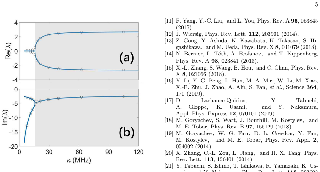
The central discovery is that a lossy cavity can be engineered into the coupling element that creates anti-PT symmetry. When the cavity mode is adiabatically eliminated under the condition that its decay rate $\kappa$ far exceeds the magnon losses and detunings, the two magnon modes obey the effective Hamiltonian $H_{\mathrm{eff}} = \begin{pmatrix} \Omega - i(\gamma+\Gamma) & -i\Gamma \\ -i\Gamma & -\Omega - i(\gamma+\Gamma) \end{pmatrix}$ with $\Omega = (\omega_1-\omega_2)/2$ and dissipative coupling $\Gamma = g^2/\kappa$. The eigenvalues $\lambda_\pm = -i(\gamma+\Gamma) \pm \sqrt{\Omega^2-\Gamma^2}$ place the exceptional point at $|\Omega| = |\Gamma|$; tuning $\kappa$ through $\kappa_0 = 15.8$ MHz moves the system from the anti-PT broken phase, where the two modes are separated, into the anti-PT phase, where the modes attract and the real parts of the eigenvalues coalesce. The authors show this transition using a magnon-readout method: reading the reflection from the two magnon antennas rather than from the cavity reveals the two magnon resonances and their attraction, whereas the cavity-readout spectrum always shows two peaks and cannot mark the exceptional point.
Load-bearing premise
The anti-PT description comes from treating the cavity as a reservoir so lossy that it can be eliminated from the equations of motion, but at the claimed transition point the cavity loss rate is only about two and a half times the magnon-cavity coupling, so the elimination is not fully justified; the description also assumes the two magnon losses and the two magnon-cavity couplings are nearly equal, which the paper states holds only to about five percent.
Editorial extensions
If this is right
- A gain-free, room-temperature platform now exists for studying anti-PT symmetry, and the exceptional point is reached simply by adjusting the cavity loss rate.
- Decreasing the cavity loss produces level attraction between the two magnon modes, the opposite of the level repulsion seen in conventional strongly coupled resonators.
- Because anti-PT systems have been proposed for enhanced exceptional-point sensing, this setup is a concrete candidate for testing such sensitivity in a magnetic system.
- Encircling the exceptional point in this system is a natural next step for observing non-adiabatic topological operations.
- The magnon-readout technique should extend to multi-magnon-cavity-polariton systems, where separately probing individual magnon modes is otherwise difficult.
Reading between the lines
- Editorial inference: the same adiabatic-elimination recipe — two modes coupled to one high-loss common reservoir — should work for other bosonic platforms such as optical or mechanical modes, making anti-PT physics as easy to build as the lossy reservoir itself.
- Editorial inference: because $\kappa_0 = 15.8$ MHz is only about $2.4\,g$ with $g \approx 6.5$ MHz, the full three-mode damped model and the anti-PT Hamiltonian are not strictly equivalent at the claimed transition; comparing the two models' eigenvalue trajectories near $\kappa_0$ would give a quantitative test of how much of the observed attraction is genuinely anti-PT.
- Editorial inference: the data could be re-fit without assuming $\gamma_1=\gamma_2$ and $g_{13}=g_{23}$; if the extracted exceptional point shifts by more than the stated five percent parameter asymmetry, the identification with the ideal anti-PT picture would need to be qualified.
- Editorial inference: adding a third magnon to the same setup may produce multi-mode anti-PT attractors or higher-order exceptional points, since the method is not restricted to two levels.
Signed reviews
Editorial analysis
A structured set of objections, weighed in public.
Referee Report
Summary. The paper reports an experimental study of two YIG magnon modes coupled through a common microwave cavity, with the cavity decay large enough that the magnons acquire an effective dissipative coupling. The authors claim that this realizes a two-dimensional anti-PT symmetric Hamiltonian, and, by tuning the cavity decay rate κ through a critical value κ0 = 15.8 MHz, they observe the spontaneous anti-PT symmetry-breaking phase transition accompanied by level attraction. The experimental evidence consists of reflection spectra S11 and S22 measured from loop antennas coupled to the two magnons (the 'magnon-readout' method), fits of these spectra to both the original three-mode Hamiltonian and the effective anti-PT Hamiltonian, and a plot of the real and imaginary parts of the eigenvalues versus κ, with the eigenvalues obtained from fitted parameters and the effective Hamiltonian. The paper also compares these magnon-readout results with conventional cavity-readout data, arguing that the cavity-readout method cannot reveal the anti-PT transition directly.
Significance. If the claims are fully supported, the work would be a useful experimental demonstration of anti-PT symmetry in a solid-state magnon-cavity platform without gain, and the magnon-readout technique could be of broader interest for probing hidden modes in multi-mode cavity polariton systems. Credit is due for the direct observation of level attraction in the raw spectra and for fitting the data to a full input-output model with a consistent set of parameters. However, the central claim of an observed anti-PT phase transition rests on eigenvalues that are reconstructed from the fitted Hamiltonian rather than extracted independently from data, and the validity of the anti-PT reduction is assessed only qualitatively. These issues need to be addressed before the observation claim can be considered established.
major comments (3)
- [Fig. 3; Supplementary Note D] The eigenvalue points in Fig. 3 are not directly measured observables. Supplementary Note D states that the system parameters are first extracted from fits to the reflection spectra and that the eigenenergies are then solved theoretically from the effective Hamiltonian. The agreement between these points and the anti-PT curves therefore partly reflects the fitted model rather than constituting an independent observation of the exceptional point. To support the central claim of an observed phase transition, the authors should either extract the complex eigenfrequencies directly from the measured S11 and S22 line shapes, for example from the poles of the response, with uncertainties, or provide a quantitative criterion applied to the raw spectra, such as the measured dip separation versus the full width at half maximum as a function of κ, with error bars that locate κ0. The current Fig. 3 has no error bars, and the text provides no uncertainty on κ0 = 15.8 MHz.
- [Supplementary Eqs. (S12)–(S18); Table I] The reduction to the anti-PT Hamiltonian Eq. (S18) requires κ much larger than |ω3 − ω1| and |ω3 − ω2|, γ1 = γ2, and g13 = g23. None of these conditions is quantified at the claimed transition point. At κ0 = 15.8 MHz with g ≈ 6.5 MHz and γ ≈ 2.2 MHz, the effective coupling is Γ = g^2/κ = 2.7 MHz; if the magnon-cavity detunings are comparable to the magnon-magnon splitting of about 5.4 MHz, the neglected real parts of the off-diagonal terms in Eq. (S16) are of order Γ times Δ/κ, which is not negligible. Moreover, Table I gives g13 = 6.65 MHz and g23 = 6.41 MHz, a difference of about 3.7 percent. The exact Hamiltonian Eq. (S16) then has unequal diagonal decay rates and complex off-diagonal couplings, which can shift the exceptional point or turn it into an avoided crossing. The authors should report the values of Δ13 and Δ23, compute the eigenvalues of Eq. (S16) with the fitted parameters, and show explicitly that a true or resolution-limited exceptional point remains at κ0 = 15.8 MHz within the experimental uncertainty.
- [Fig. 2(a) and Fig. S1; main text near 'Using the definition of EP'] The only direct spectral evidence for the transition is the merging of the dips in S11 and S22 as κ is reduced. The text states that in the broken phase the dip separation is larger than the FWHM and in the symmetric phase it is smaller, but no measured values, fits to the dip positions, or uncertainties are given, and the combined spectrum S̄ = (S11 + S22)/2 is acknowledged in Supplementary Note C not to correspond to a physical observable. Consequently the value κ0 = 15.8 MHz is not located by a quantitative criterion applied to the raw data; it is effectively the value at which the reconstructed eigenvalues of the fitted model cross. Please provide the measured dip separation and the FWHM versus κ, or another observable-based estimator, with uncertainties.
minor comments (5)
- [Supplementary Eqs. (S26)–(S28)] Equations (S26) and (S27) are printed identically; if this is not a typo, the text should explain why aout and cout are the same and why the total reflection coefficient is their average.
- [Main text, first paragraph] 'Kittle mode' should be 'Kittel mode'.
- [Conclusion] 'couped' should be 'coupled' in the sentence 'the unique ability of magnon-readout method in exploring multi-magnon-cavity couped systems'.
- [Fig. S2 caption] 'theorectical' should be 'theoretical'.
- [Supplementary Note B] The statement that 'there are only fitting parameters ϕ13 or ϕ23' is not reconciled with the many parameters listed in Table I; please clarify which parameters are independently calibrated and which are fitted.
Circularity Check
Fig. 3 eigenvalue curves are computed from the effective anti-PT Hamiltonian with fitted parameters, so the 'observed' transition partly reduces to a consistency check rather than an independent measurement.
-
fitted input called prediction
[Main text, eigenvalue discussion around Fig. 3; Supplementary Note D]
"Using the method elaborated in Supplementary Material D, we extract the eigenvalues and plot the real and imaginary parts as a function of κ in FIG. 3 (a) and (b) respectively, which show excellent agreement with theoretical results. The experimental data in FIG. 3 (a) reveal that the exceptional point occurs at κ0 = 15.8 MHz"
Supplementary Note D defines the 'extraction' as: 'we experimentally obtain the parameters of the system and theoretically solve the eigenenergies using the following Hamiltonian' (Eq. S16), and 'The fitting lines in Fig. 4 are drawn with the mean value of the corresponding parameters with the anti-PT Hamiltonian Eq. S18.' Eq. S16/S18 is the same effective anti-PT Hamiltonian whose eigenvalues are presented as the predicted result, and its input parameters are obtained from fits to the measured spectra. Therefore the Fig. 3 curves are model outputs evaluated at fitted parameters, not independently measured eigenvalues; the 'excellent agreement' is partly a consistency check of the fitted model rather than an observation of the exceptional point.
full rationale
The derivation of the effective anti-PT Hamiltonian in Supplementary A is a legitimate adiabatic elimination from the original Hamiltonian (Eqs. S12-S18), not circular with respect to the anti-PT claim: the anti-PT form follows from explicitly stated conditions (κ ≫ γ, κ ≫ |Δ13|, |Δ23|, γ1 ≈ γ2, g13 ≈ g23). No load-bearing self-citation or imported uniqueness theorem was found; Ref. [11] supplies the anti-PT form externally, and the approximations are stated rather than hidden. The main circularity burden is the eigenvalue 'observation' in Fig. 3: those curves are generated by solving the effective Hamiltonian with Table I parameters fitted from the raw spectra, so they cannot independently confirm the anti-PT phase transition. Some independent grounding remains because the raw S11/S22 and combined spectra directly show dip merging and level attraction, although the FWHM-based EP criterion is not quantified against those raw data. The finite-κ corrections at κ0 = 15.8 MHz and the few-percent asymmetries in g13/g23 and γ1/γ2 are correctness risks, not additional circularity.
Assumptions & free parameters
free parameters (10)
- g13 =
6.65 MHz (magnon-readout); 9.77 MHz (cavity-readout)
- g23 =
6.41 MHz (magnon-readout); 9.61 MHz (cavity-readout)
- gamma1 =
2.22 MHz (magnon-readout); 1.11 MHz (cavity-readout)
- gamma2 =
2.22 MHz (magnon-readout); 1.11 MHz (cavity-readout)
- kappa_int =
1.5 MHz
- kappa1 =
0.45 MHz
- kappa2 =
0.92 MHz
- kappa3 =
tunable
- phi13 =
fitted
- phi23 =
fitted
assumptions (6)
- domain assumption The two YIG spheres are in the low-excitation regime and their magnon modes are linear harmonic resonators.
- standard math Standard Markovian input-output theory with Langevin equations describes the antenna-magnon-cavity system.
- domain assumption The cavity mode can be adiabatically eliminated because kappa is large enough.
- domain assumption The two magnon damping rates and the two magnon-cavity couplings are equal.
- domain assumption The coupling phases Phi_13 and Phi_23 are negligible.
- domain assumption There is no direct magnon-magnon interaction; the two YIG spheres couple only through the cavity mode.
Cite this review
Pith. "Pith review of Observation of anti-PT symmetry phase transition in the magnon-cavity-magnon coupled system." pith.science (2026). https://pith.science/paper/N7ZT43ZX
@misc{pith2026190803358,
  author       = {Pith},
  title        = {Pith review of: Observation of anti-PT symmetry phase transition in the magnon-cavity-magnon coupled system},
  year         = {2026},
  howpublished = {\url{https://pith.science/paper/N7ZT43ZX}},
  note         = {Machine review of arXiv:1908.03358}
}
read the original abstract
As the counterpart of PT symmetry, abundant phenomena and potential applications of anti-PT symmetry have been predicted or demonstrated theoretically. However, experimental realization of the coupling required in the anti-PT symmetry is difficult. Here, by coupling two YIG spheres to a microwave cavity, the large cavity dissipation rate makes the magnons coupled dissipatively with each other, thereby obeying a two-dimensional anti-PT Hamiltonian. In terms of the magnon-readout method, a new method adopted here, we demonstrate the validity of our method in constructing an anti-PT system and present the counterintuitive level attraction process. Our work provides a new platform to explore the anti-PT symmetry properties and paves the way to study multi-magnoncavity-polariton systems.
Figures


Reference graph
Works this paper leans on
-
[1]
de Vega and D
I. de Vega and D. Alonso, Rev. Mod. Phys. 89, 015001 (2017)
2017
- [2]
-
[3]
Miri and A
M.-A. Miri and A. Al` u, Science 363, eaar7709 (2019)
2019
-
[4]
El-Ganainy, K
R. El-Ganainy, K. G. Makris, M. Khajavikhan, Z. H. Musslimani, S. Rotter, and D. N. Christodoulides, Nat. Phys. 14, 11 (2018)
2018
-
[5]
L. Feng, R. El-Ganainy, and L. Ge, Nat. Photonics 11, 752 (2017)
2017
- [6]
-
[7]
Y. Wu, W. Liu, J. Geng, X. Song, X. Ye, C.-K. Duan, X. Rong, and J. Du, Science 364, 878 (2019), https://science.sciencemag.org/content/364/6443/878.full.pdf
work page 2019
-
[8]
P. Peng, W. Cao, C. Shen, W. Qu, J. Wen, L. Jiang, and Y. Xiao, Nat. Phys. 12, 1139 (2016)
work page 2016
Show all 42 references
-
[9]
Y. Choi, C. Hahn, J. W. Yoon, and S. H. Song, Nat. Commun. 9, 2182 (2018)
2018
-
[10]
Lau and A
H.-K. Lau and A. A. Clerk, Nat. Commun. 9, 4320 (2018)
2018
-
[11]
(Supplementary Materials A): Heff = [Ω − i(γ + Γ) −iΓ −iΓ −Ω − i(γ + Γ) ] . (1) Here iΓ is the dissipative coupling rate, Ω = ( ω1 − ω2)/2 is the effective detuning in the rotating reference frame with frequency ( ω1 + ω2)/2, where ω1 (ω2) is the reso- nant frequency of magnon 1...
-
[12]
Yang, Y.-C
F. Yang, Y.-C. Liu, and L. You, Phys. Rev. A 96, 053845 (2017)
2017
-
[13]
Wiersig, Phys
J. Wiersig, Phys. Rev. Lett. 112, 203901 (2014)
2014
-
[14]
Z. Gong, Y. Ashida, K. Kawabata, K. Takasan, S. Hi- gashikawa, and M. Ueda, Phys. Rev. X 8, 031079 (2018)
2018
-
[15]
Bernier, L
N. Bernier, L. T´ oth, A. Feofanov, and T. Kippenberg, Phys. Rev. A 98, 023841 (2018)
2018
-
[16]
Zhang, S
X.-L. Zhang, S. Wang, B. Hou, and C. Chan, Phys. Rev. X 8, 021066 (2018)
2018
-
[17]
Li, Y.-G
Y. Li, Y.-G. Peng, L. Han, M.-A. Miri, W. Li, M. Xiao, X.-F. Zhu, J. Zhao, A. Al` u, S. Fan, et al. , Science 364, 170 (2019)
2019
-
[18]
Lachance-Quirion, Y
D. Lachance-Quirion, Y. Tabuchi, A. Gloppe, K. Usami, and Y. Nakamura, Appl. Phys. Express 12, 070101 (2019)
2019
-
[19]
Goryachev, S
M. Goryachev, S. Watt, J. Bourhill, M. Kostylev, and M. E. Tobar, Phys. Rev. B 97, 155129 (2018)
2018
-
[20]
Goryachev, W
M. Goryachev, W. G. Farr, D. L. Creedon, Y. Fan, M. Kostylev, and M. E. Tobar, Phys. Rev. Appl. 2, 054002 (2014)
2014
-
[21]
Zhang, C.-L
X. Zhang, C.-L. Zou, L. Jiang, and H. X. Tang, Phys. Rev. Lett. 113, 156401 (2014)
2014
-
[22]
Tabuchi, S
Y. Tabuchi, S. Ishino, T. Ishikawa, R. Yamazaki, K. Us- ami, and Y. Nakamura, Phys. Rev. Lett. 113, 083603 (2014)
2014
-
[23]
Zhang, X.-M
D. Zhang, X.-M. Wang, T.-F. Li, X.-Q. Luo, W. Wu, F. Nori, and J. You, npj Quantum Inf. 1, 15014 (2015)
2015
-
[24]
Zhang, C
X. Zhang, C. Zou, L. Jiang, and H. X. Tang, J. Appl. Phys. 119, 023905 (2016)
2016
-
[25]
Bourhill, N
J. Bourhill, N. Kostylev, M. Goryachev, D. Creedon, and M. Tobar, Phys. Rev. B 93, 144420 (2016)
2016
-
[26]
Zhang, C.-L
X. Zhang, C.-L. Zou, N. Zhu, F. Marquardt, L. Jiang, and H. X. Tang, Nat. Commun. 6, 8914 (2015)
2015
-
[27]
B. Z. Rameshti and G. E. Bauer, Phys. Rev. B 97, 014419 (2018)
2018
-
[28]
N. J. Lambert, J. Haigh, S. Langenfeld, A. Doherty, and A. Ferguson, Phys. Rev. A 93, 021803 (2016)
2016
-
[29]
Zhang and J
G.-Q. Zhang and J. You, Phys. Rev. B 99, 054404 (2019)
2019
-
[30]
Zhang, X.-Q
D. Zhang, X.-Q. Luo, Y.-P. Wang, T.-F. Li, and J. You, Nat. Commun. 8, 1368 (2017)
2017
-
[31]
Tabuchi, S
Y. Tabuchi, S. Ishino, A. Noguchi, T. Ishikawa, R. Ya- mazaki, K. Usami, and Y. Nakamura, Science 349, 405 (2015)
2015
-
[32]
Lachance-Quirion, Y
D. Lachance-Quirion, Y. Tabuchi, S. Ishino, A. Noguchi , T. Ishikawa, R. Yamazaki, and Y. Nakamura, Sci. Adv. 3, e1603150 (2017)
2017
-
[33]
S. V. Kusminskiy, H. X. Tang, and F. Marquardt, Phys. Rev. A 94, 033821 (2016)
2016
-
[34]
Hisatomi, A
R. Hisatomi, A. Osada, Y. Tabuchi, T. Ishikawa, A. Noguchi, R. Yamazaki, K. Usami, and Y. Nakamura, Phys. Rev. B 93, 174427 (2016)
2016
-
[35]
Zhang, N
X. Zhang, N. Zhu, C.-L. Zou, and H. X. Tang, Phys. Rev. Lett. 117, 123605 (2016)
2016
-
[36]
J. Graf, H. Pfeifer, F. Marquardt, and S. V. Kusminskiy, Phys. Rev. B 98, 241406 (2018)
2018
-
[37]
Holanda, D
J. Holanda, D. Maior, A. Azevedo, and S. Rezende, Nat. Phys. 14, 500 (2018)
2018
-
[38]
Zhang, C.-L
X. Zhang, C.-L. Zou, L. Jiang, and H. X. Tang, Sci. Adv. 2, e1501286 (2016). arXiv:1908.03358v1 [quant-ph] 9 Aug 2019 Supplementary Materials for Observation of anti- PT symmetry phase transition in the magnon-cavity-magnon coupled syst em Jie Zhao, 1, 2, 3, ∗ Yulong Liu, 4, ∗...
2016 arXiv
-
[39]
Yang, Y.-C
F. Yang, Y.-C. Liu, and L. You, Physical Review A 96, 053845 (2017)
2017
-
[40]
Harder, Y
M. Harder, Y. Yang, B. M. Yao, C. H. Yu, J. W. Rao, Y. S. Gui, R . L. Stamps, and C.-M. Hu, Phys. Rev. Lett. 121, 137203 (2018)
2018
-
[41]
D. F. Walls and G. J. Milburn, Quantum optics (Springer Science & Business Media, 2007)
2007
-
[42]
A. A. Clerk, M. H. Devoret, S. M. Girvin, F. Marquardt, and R. J. Schoelkopf, Reviews of Modern Physics 82, 1155 (2010). 9 FIG. S2. color online. The reflection coefficient spectra S 33 read from the antenna 3 with different cavity dissipation rates. The black dot are experiment d...
2010
Reviewed August 14, 2026 · model on record in the stance chip above.
Discussion (0). Continue with ORCID to comment.