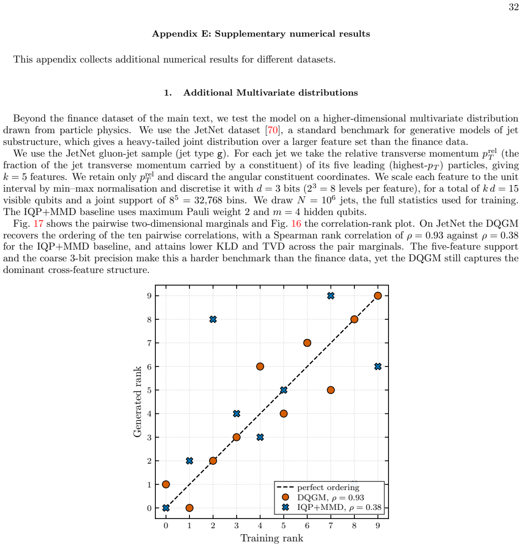
Quantum Fourier Generative Models Trainable at Large Scale
Pith reviewed 2026-06-30 01:22 UTC · model grok-4.3
The pith
Quantum generative models train classically at over 1000 qubits using Fourier feature maps and a Parseval-based log-likelihood estimator, then deploy to quantum hardware for sampling.
A machine-rendered reading of the paper's core claim, the machinery that carries it, and where it could break.
Core claim
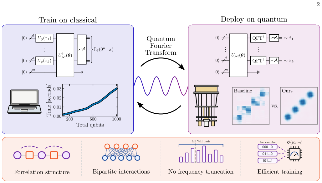
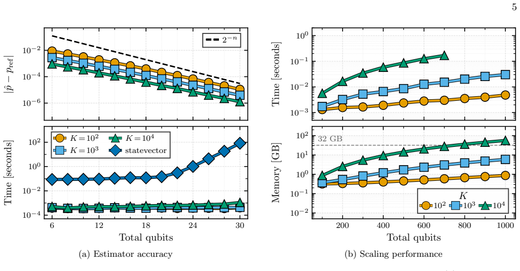
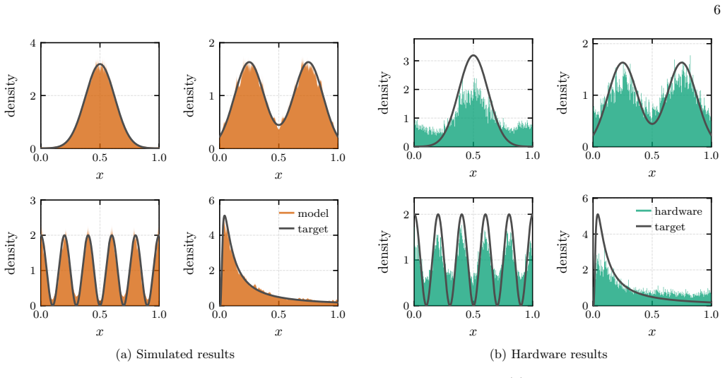
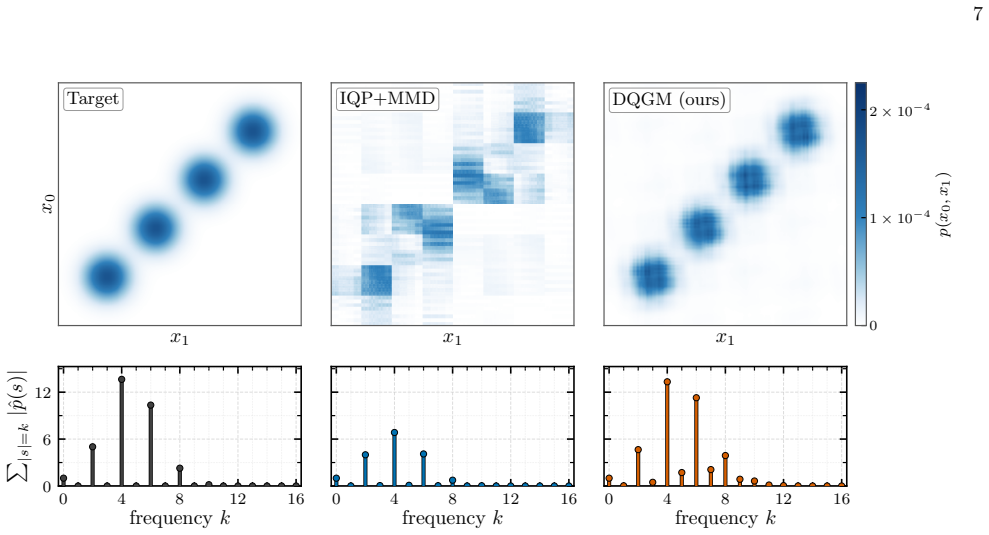
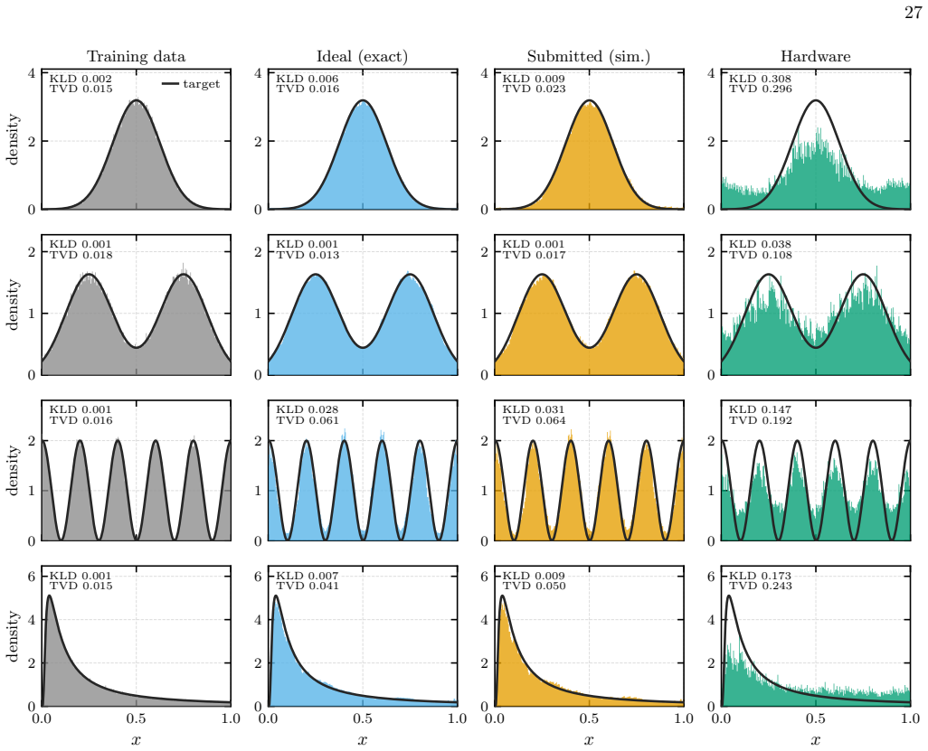
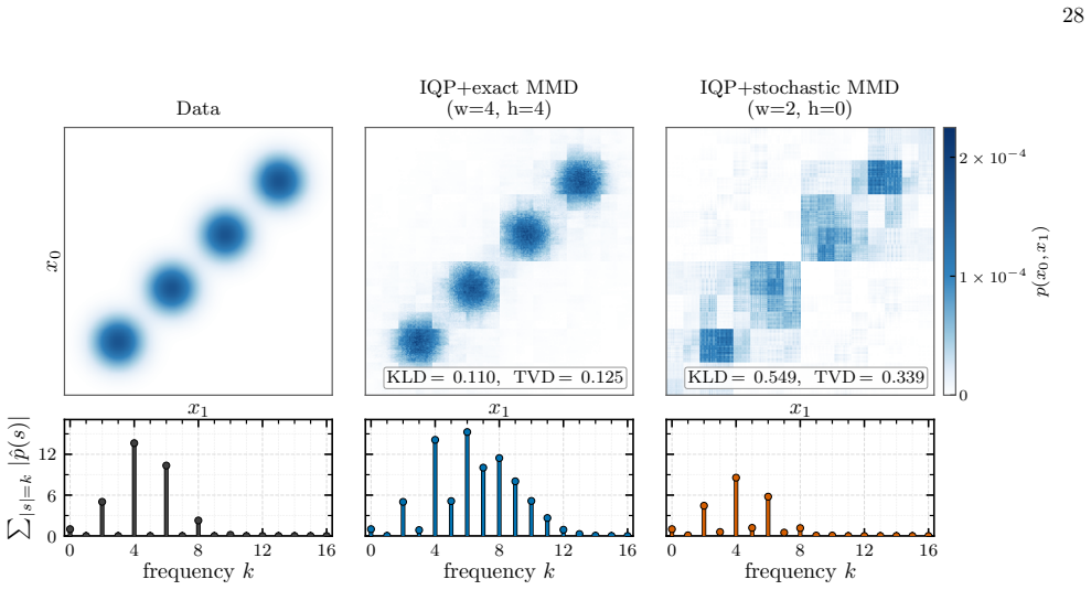
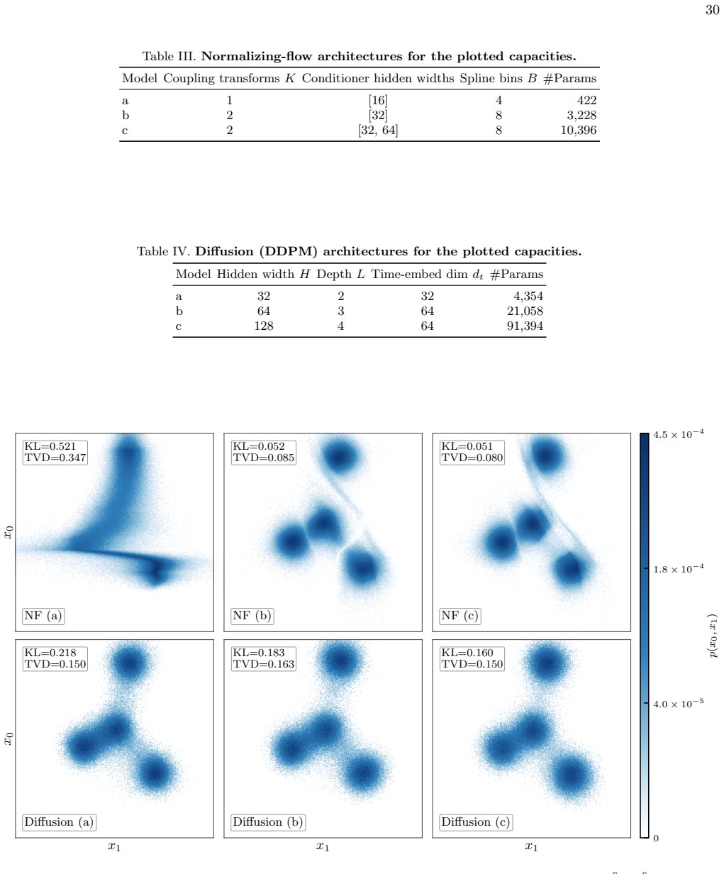
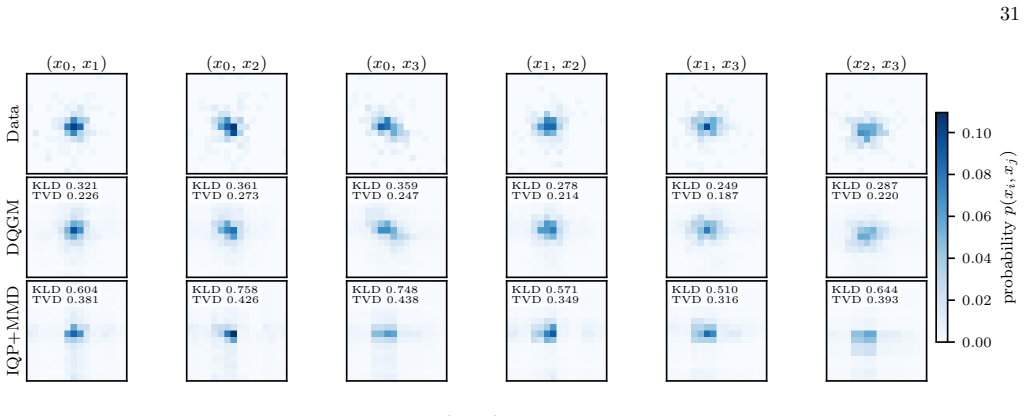
By combining parallel Fourier feature maps for embedding with forrelation-type circuits and training on an unbiased Monte Carlo estimator of log-likelihood loss obtained from Parseval's identity, quantum generative models can be trained at scales over 1000 qubits on classical hardware; once trained, inverse quantum Fourier transforms map the model to a separate sampling circuit in the computational basis that runs on quantum devices, achieving low total variation distance while avoiding the oversmoothing seen in classical baselines.
What carries the argument
The unbiased Monte Carlo estimator of log-likelihood loss derived from Parseval's identity applied to Fourier feature maps and forrelation circuits, which enables tractable classical training at large scale before inverse-QFT mapping to a sampling circuit.
If this is right
- Univariate and bivariate models with highly non-trivial structure reach low total variation distance to the target.
- The trained models avoid oversmoothing and preserve multi-modal structure better than normalizing flow or diffusion baselines.
- Fine-tuned IQP circuits trained with MMD loss perform poorly by comparison.
- Deployed models achieve per-sample execution times of approximately 300 microseconds on superconducting quantum hardware.
Where Pith is reading between the lines
- The separation of classical training from quantum sampling phases could allow the same framework to target higher-dimensional distributions if the estimator's scaling holds.
- Fast per-sample quantum execution times open the possibility of using these models for real-time inference tasks that require many draws from complex distributions.
- If the Fourier embedding generalizes, the approach might serve as a template for other quantum generative tasks where moment-matching losses have previously limited expressivity.
Load-bearing premise
The log-likelihood loss estimator based on Parseval's identity remains unbiased and computationally tractable for the chosen Fourier feature maps and forrelation circuits at the reported qubit counts without hidden dependence on post-hoc parameter choices.
What would settle it
Running exact log-likelihood computation on a 10-qubit instance of the same Fourier feature map and forrelation circuit and finding that the Monte Carlo estimator deviates by more than statistical error would falsify the claim of unbiased scalability.
Figures
read the original abstract
We propose an algorithmic framework for building and training quantum generative models corresponding to multivariate probability distributions. Our model uses parallel Fourier feature maps for embedding continuous-valued variables combined with a forrelation-type quantum circuit for tuning Fourier coefficients of the quantum model. Crucially, we develop a distinct training strategy where training is enabled at large scale by log-likelihood loss with unbiased Monte Carlo estimator based on Parseval's identity. Unlike prior work that relied on maximal mean discrepancy (MMD) loss, our approach goes beyond matching just low frequency moments, while enabling efficient classical training. Once the model is trained, we use inverse quantum Fourier transforms to map it into a separate sampling circuit in the computational basis. We demonstrate the efficiency of the suggested framework by validating loss estimation at the scale of over 1000 qubits on a single GPU. We show that univariate and bivariate models with highly non-trivial structure can be trained to low total variation distance, while fine-tuned IQP models with MMD loss show poor performance. Comparing to classical baselines represented by normalizing flow and diffusion models, we show that our approach avoids oversmoothing and preserves multi-modal structure of the target. Finally, we have deployed the trained models on superconducting quantum devices, successfully sampling distributions with per-sample execution times of approximately $300\,\mu\mathrm{s}$. Our work shows that quantum generative models with the train-on-classical deploy-on-quantum approach can provide both high-quality structure at increased scale and fast sampling access needed for inference.
Editorial analysis
A structured set of objections, weighed in public.
Referee Report
Summary. The paper proposes an algorithmic framework for quantum generative models of multivariate distributions. It combines parallel Fourier feature maps for continuous variables with a forrelation-type circuit to tune Fourier coefficients. A key contribution is a log-likelihood training objective whose unbiased Monte Carlo estimator is derived from Parseval's identity, enabling classical training at scales exceeding 1000 qubits on a single GPU. After training, an inverse quantum Fourier transform produces a sampling circuit in the computational basis. Experiments report low total-variation distance for univariate and bivariate targets with non-trivial structure, superior performance relative to MMD-tuned IQP circuits and classical normalizing-flow/diffusion baselines (avoiding oversmoothing), and deployment on superconducting hardware with ~300 μs per-sample times.
Significance. If the Parseval-based estimator is confirmed to be unbiased and to possess tractable variance independent of the fitted model, the work would demonstrate a concrete route to classically trainable quantum generative models that scale beyond current MMD-limited approaches while preserving multi-modal structure. The train-on-classical/deploy-on-quantum separation and the reported hardware sampling times would constitute a practical advantage over purely classical or purely quantum generative methods at the claimed qubit counts.
major comments (2)
- [Methods / loss estimator] The central scalability claim (loss estimation and training at >1000 qubits) rests on the Monte Carlo estimator derived from Parseval's identity remaining unbiased and having variance that does not grow prohibitively with the number of Fourier modes or the forrelation circuit depth. The abstract provides no explicit variance bound, circuit-depth scaling, or proof that the estimator is independent of post-hoc parameter choices; this must be supplied with a concrete derivation or numerical verification in the methods section before the efficiency result can be accepted.
- [Experiments] The comparison to fine-tuned IQP models with MMD loss reports poor performance, yet the paper does not specify the circuit depth, number of Fourier modes, or optimization hyperparameters used for the IQP baseline. Without these controls it is impossible to determine whether the reported advantage is due to the loss function, the feature-map architecture, or differences in model capacity.
minor comments (2)
- [Abstract] The abstract states that models are trained to low total variation distance, but no numerical values, error bars, or dataset sizes are given; these should appear in the results tables or figures.
- [Model definition] Notation for the parallel Fourier feature maps and the forrelation unitary should be introduced with explicit definitions of the feature dimension and the circuit's action on the Fourier coefficients.
Simulated Author's Rebuttal
We thank the referee for the careful review and constructive comments. We respond to each major comment below, indicating where we will revise the manuscript to address the concerns.
read point-by-point responses
-
Referee: [Methods / loss estimator] The central scalability claim (loss estimation and training at >1000 qubits) rests on the Monte Carlo estimator derived from Parseval's identity remaining unbiased and having variance that does not grow prohibitively with the number of Fourier modes or the forrelation circuit depth. The abstract provides no explicit variance bound, circuit-depth scaling, or proof that the estimator is independent of post-hoc parameter choices; this must be supplied with a concrete derivation or numerical verification in the methods section before the efficiency result can be accepted.
Authors: The methods section already derives the unbiased estimator from Parseval's identity and demonstrates numerical stability at >1000 qubits. We agree, however, that an explicit variance analysis is needed to fully support the scalability claim. In the revised manuscript we will add a derivation showing that the estimator variance depends only on the number of Monte Carlo samples (and is independent of forrelation depth and Fourier-mode count) together with additional numerical verification of variance scaling. revision: yes
-
Referee: [Experiments] The comparison to fine-tuned IQP models with MMD loss reports poor performance, yet the paper does not specify the circuit depth, number of Fourier modes, or optimization hyperparameters used for the IQP baseline. Without these controls it is impossible to determine whether the reported advantage is due to the loss function, the feature-map architecture, or differences in model capacity.
Authors: We acknowledge the omission of these controls. The revised experiments section will explicitly state the circuit depth, number of Fourier modes, and optimization hyperparameters employed for the MMD-tuned IQP baselines, enabling a clear assessment that the observed performance gap arises from the loss function and architecture rather than unequal model capacity. revision: yes
Circularity Check
No significant circularity; estimator grounded in external theorem
full rationale
The paper's training strategy relies on a log-likelihood estimator derived via Parseval's identity (a standard external theorem) applied to the Fourier feature map model. This is used to enable classical training of parameters in the forrelation circuit, followed by separate inverse QFT sampling. No load-bearing step reduces by construction to fitted inputs, self-definition, or self-citation chains. The scalability demonstration at >1000 qubits is presented as empirical validation rather than a derived equivalence. The derivation chain remains self-contained against external mathematical facts and does not exhibit the enumerated circular patterns.
Axiom & Free-Parameter Ledger
free parameters (1)
- Fourier coefficients
axioms (1)
- domain assumption Parseval's identity applies directly to the quantum Fourier feature map and forrelation circuit to yield an unbiased Monte Carlo estimator of log-likelihood.
invented entities (1)
-
Quantum Fourier generative model with parallel feature maps and forrelation circuit
no independent evidence
Reference graph
Works this paper leans on
-
[1]
Generalized Denoising Auto-Encoders as Generative Models
Y. Bengio, L. Yao, G. Alain, and P. Vincent, General- ized denoising auto-encoders as generative models (2013), arXiv:1305.6663 [cs.LG]
work page internal anchor Pith review Pith/arXiv arXiv 2013
-
[2]
Rezende and S
D. Rezende and S. Mohamed, inProceedings of the 32nd International Conference on Machine Learning, Proceed- ings of Machine Learning Research, Vol. 37, edited by F. Bach and D. Blei (PMLR, Lille, France, 2015) pp. 1530–1538
2015
-
[3]
J. Song, C. Meng, and S. Ermon, inInternational Con- ference on Learning Representations(2021)
2021
-
[4]
Y. Song, J. Sohl-Dickstein, D. P. Kingma, A. Kumar, S. Ermon, and B. Poole, inInternational Conference on Learning Representations(2021)
2021
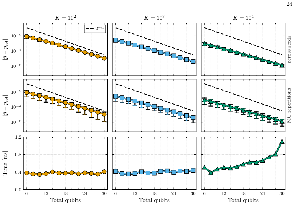
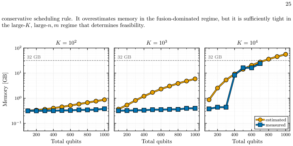
-
[5]
Liu and L
J.-G. Liu and L. Wang, Phys. Rev. A98, 062324 (2018)
2018
-
[6]
Zoufal, A
C. Zoufal, A. Lucchi, and S. Woerner, npj Quantum In- formation5, 103 (2019)
2019
-
[7]
Coyle, D
B. Coyle, D. Mills, V. Danos, and E. Kashefi, npj Quan- tum Information6, 60 (2020)
2020
- [8]
-
[9]
Aaronson and A
S. Aaronson and A. Arkhipov, Theory of Computing9, 143 (2013)
2013
-
[10]
Arute, K
F. Arute, K. Arya, R. Babbush, D. Bacon, J. C. Bardin, R. Barends, R. Biswas, S. Boixo, F. G. S. L. Brandao, D. A. Buell, and et al., Nature574, 505 (2019)
2019
-
[11]
Hangleiter and J
D. Hangleiter and J. Eisert, Rev. Mod. Phys.95, 035001 (2023)
2023
- [12]
-
[13]
M. H. Amin, E. Andriyash, J. Rolfe, B. Kulchytskyy, and R. Melko, Physical Review X8, 021050 (2018)
2018
-
[14]
Coopmans and M
L. Coopmans and M. Benedetti, Communications Physics7, 274 (2024)
2024
-
[15]
C. T¨ uys¨ uz, M. Demidik, L. Coopmans, E. Rinaldi, V. Croft, Y. Haddad, M. Rosenkranz, and K. Jansen, Learning to generate high-dimensional distributions with low-dimensional quantum boltzmann machines (2024), arXiv:2410.16363 [quant-ph]
-
[16]
Demidik, C
M. Demidik, C. T¨ uys¨ uz, N. Piatkowski, M. Grossi, and K. Jansen, Communications Physics8, 413 (2025)
2025
-
[17]
M. Demidik, C. T¨ uys¨ uz, M. Grossi, and K. Jansen, Sample-based training of quantum generative models (2025), arXiv:2511.11802 [quant-ph]
-
[18]
Kyriienko, A
O. Kyriienko, A. E. Paine, and V. E. Elfving, Physical Review Research6, 033291 (2024)
2024
-
[19]
A. E. Paine, V. E. Elfving, and O. Kyriienko, Advanced Quantum Technologies6, 2300065 (2023)
2023
-
[20]
Bak´ o, D
B. Bak´ o, D. T. R. Nagy, P. H´ aga, Z. Kallus, and Z. Zim- bor´ as, Quantum Science and Technology11, 035012 (2026)
2026
-
[21]
Oszmaniec, N
M. Oszmaniec, N. Dangniam, M. E. Morales, and Z. Zim- bor´ as, PRX Quantum3, 020328 (2022)
2022
-
[22]
Y. Wang, S. Xue, Y. Wang, Y. Liu, J. Ding, W. Shi, D. Wang, Y. Liu, X. Fu, G. Huang, A. Huang, M. Deng, and J. Wu, Opt. Lett.48, 5197 (2023)
2023
-
[23]
R. Kailasanathan, W. R. Clements, M. R. Bosk- abadi, S. M. Gibford, E. Papadakis, C. J. Savoie, and S. S. Mansouri, Quantum enhanced ensemble gans for anomaly detection in continuous biomanufacturing (2026), arXiv:2508.21438 [cs.LG]
-
[24]
Quantum latent distributions in deep generative models
O. Bacarreza, T. Farnsworth, A. Makarovskiy, H. Wall- ner, T. Hicks, S. Sempere-Llagostera, J. Price, R. J. A. Francis-Jones, and W. R. Clements, Quantum la- tent distributions in deep generative models (2026), arXiv:2508.19857 [cs.LG]
work page internal anchor Pith review Pith/arXiv arXiv 2026
- [25]
-
[26]
Holmes, K
Z. Holmes, K. Sharma, M. Cerezo, and P. J. Coles, PRX Quantum3, 010313 (2022)
2022
-
[27]
Cerezo, M
M. Cerezo, M. Larocca, D. Garc´ ıa-Mart´ ın, N. L. Diaz, P. Braccia, E. Fontana, M. S. Rudolph, P. Bermejo, A. Ijaz, S. Thanasilp, E. R. Anschuetz, and Z. Holmes, Nature Communications16, 7907 (2025)
2025
-
[28]
J. R. McClean, S. Boixo, V. N. Smelyanskiy, R. Babbush, and H. Neven, Nature Communications9, 4812 (2018)
2018
-
[29]
Larocca, S
M. Larocca, S. Thanasilp, S. Wang, K. Sharma, J. Bia- monte, P. J. Coles, L. Cincio, J. R. McClean, Z. Holmes, and M. Cerezo, Nature Reviews Physics7, 174 (2025)
2025
-
[30]
X. You and X. Wu, Exponentially many local minima in quantum neural networks (2021), arXiv:2110.02479 [quant-ph]
- [31]
-
[32]
Schuld, V
M. Schuld, V. Bergholm, C. Gogolin, J. Izaac, and N. Kil- loran, Phys. Rev. A99, 032331 (2019)
2019
-
[33]
Kyriienko and V
O. Kyriienko and V. E. Elfving, Phys. Rev. A104, 052417 (2021)
2021
-
[34]
Wierichs, J
D. Wierichs, J. Izaac, C. Wang, and C. Y.-Y. Lin, Quan- tum6, 677 (2022)
2022
-
[35]
Kasture, O
S. Kasture, O. Kyriienko, and V. E. Elfving, Phys. Rev. A108, 042406 (2023)
2023
-
[36]
E. Recio-Armengol, S. Ahmed, and J. Bowles, Train on classical, deploy on quantum: scaling generative quantum machine learning to a thousand qubits (2026), arXiv:2503.02934 [quant-ph]
- [37]
- [38]
-
[39]
Z. Kolarovszki, B. Bak´ o, M. Oszmaniec, C. Oh, and Z. Zimbor´ as, Generative modeling with gaussian boson sampling: classically trainable bosonic born machines (2026), arXiv:2603.11195 [quant-ph]
-
[40]
F. Gottlieb, R. Mezher, B. Ventura, S. Mansfield, and A. Salavrakos, Efficient training of photonic quantum generative models (2026), arXiv:2603.08793 [quant-ph]
- [41]
-
[42]
M. V. den Nest, Simulating quantum computers with probabilistic methods (2010), arXiv:0911.1624 [quant- 12 ph]
work page internal anchor Pith review Pith/arXiv arXiv 2010
-
[43]
M. S. Rudolph, S. Lerch, S. Thanasilp, O. Kiss, O. Shaya, S. Vallecorsa, M. Grossi, and Z. Holmes, npj Quantum Information10, 116 (2024)
2024
-
[44]
Spectral methods: crucial for machine learning, natural for quantum computers?
V. Belis, J. Bowles, R. Gupta, E. Peters, and M. Schuld, Spectral methods: crucial for machine learning, natu- ral for quantum computers? (2026), arXiv:2603.24654 [quant-ph]
work page internal anchor Pith review Pith/arXiv arXiv 2026
-
[45]
M. Herrero-Gonzalez, B. Coyle, K. McDowall, R. Grassie, S. Beentjes, A. Khamseh, and E. Kashefi, The born ultimatum: Conditions for classical surrogation of quantum generative models with correlators (2025), arXiv:2511.01845 [quant-ph]
- [46]
-
[47]
D. Wakeham and M. Schuld, Inference, interference and invariance: How the quantum fourier transform can help to learn from data (2024), arXiv:2409.00172 [quant-ph]
-
[48]
Di Meglio, K
A. Di Meglio, K. Jansen, I. Tavernelli,et al., PRX Quan- tum5, 037001 (2024)
2024
-
[49]
Aaronson and A
S. Aaronson and A. Ambainis, SIAM Journal on Com- puting47, 982 (2018)
2018
-
[50]
Umeano, S
C. Umeano, S. Scali, and O. Kyriienko, Phys. Rev. A 113, 052425 (2026)
2026
- [51]
-
[52]
G. E. Hinton, A practical guide to training restricted boltzmann machines, inNeural Networks: Tricks of the Trade: Second Edition, edited by G. Montavon, G. B. Orr, and K.-R. M¨ uller (Springer Berlin Heidelberg, Berlin, Heidelberg, 2012) pp. 599–619
2012
-
[53]
Demonstrating Record Fidelity for the Quantum Fourier Transform
P. Aumann, M. Fellner, D. Alber, M. Cykiert, C. Flecken- stein, R. ter Hoeven, L. Stenzel, R. J. Valencia-Tortora, and W. Lechner, Demonstrating record fidelity for the quantum fourier transform (2026), arXiv:2604.12465 [quant-ph]
work page internal anchor Pith review Pith/arXiv arXiv 2026
-
[54]
T¨ uys¨ uzet al.,https://github.com/cnktysz/DQGM (2026), GitHub repository
C. T¨ uys¨ uzet al.,https://github.com/cnktysz/DQGM (2026), GitHub repository
2026
-
[55]
C. T¨ uys¨ uzet al.,https://doi.org/10.6084/m9. figshare.32789952(2026), Public dataset repository
work page doi:10.6084/m9 2026
-
[56]
M. A. Nielsen and I. L. Chuang,Quantum Computation and Quantum Information, 10th ed. (Cambridge Univer- sity Press, 2010)
2010
- [57]
-
[58]
H.-Y. Wu, V. E. Elfving, and O. Kyriienko, Advanced Quantum Technologies8, 2400337 (2025)
2025
-
[59]
J. J. Mart´ ınez de Lejarza, H.-Y. Wu, O. Kyriienko, G. Rodrigo, and M. Grossi, Communications Physics8, 448 (2025)
2025
-
[60]
D. Shepherd and M. J. Bremner, Proceedings of the Royal Society A: Mathematical, Physi- cal and Engineering Sciences465, 1413 (2009), https://royalsocietypublishing.org/rspa/article- pdf/465/2105/1413/753599/rspa.2008.0443.pdf
-
[61]
M. J. Bremner, A. Montanaro, and D. J. Shepherd, Phys. Rev. Lett.117, 080501 (2016)
2016
-
[62]
Aaronson, inProceedings of the Forty-Second ACM Symposium on Theory of Computing, STOC ’10 (Asso- ciation for Computing Machinery, New York, NY, USA,
S. Aaronson, inProceedings of the Forty-Second ACM Symposium on Theory of Computing, STOC ’10 (Asso- ciation for Computing Machinery, New York, NY, USA,
-
[63]
O’Donnell,Analysis of Boolean Functions(Cambridge University Press, USA, 2014)
R. O’Donnell,Analysis of Boolean Functions(Cambridge University Press, USA, 2014)
2014
-
[64]
A. Javadi-Abhari, M. Treinish, K. Krsulich, C. J. Wood, J. Lishman, J. Gacon, S. Martiel, P. D. Nation, L. S. Bishop, A. W. Cross, B. R. Johnson, and J. M. Gambetta, Quantum computing with Qiskit (2024), arXiv:2405.08810 [quant-ph]
work page internal anchor Pith review Pith/arXiv arXiv 2024
-
[65]
Akiba, S
T. Akiba, S. Sano, T. Yanase, T. Ohta, and M. Koyama, inProceedings of the 25th ACM SIGKDD International Conference on Knowledge Discovery and Data Mining (2019)
2019
-
[66]
Durkan, A
C. Durkan, A. Bekasov, I. Murray, and G. Papamakar- ios, inProceedings of the 33rd International Conference on Neural Information Processing Systems(Curran As- sociates Inc., Red Hook, NY, USA, 2019)
2019
-
[67]
Rozet and others, Zuko: Normalizing flows in pytorch (2024)
F. Rozet and others, Zuko: Normalizing flows in pytorch (2024)
2024
-
[68]
Paszke, S
A. Paszke, S. Gross, F. Massa, A. Lerer, J. Bradbury, G. Chanan, T. Killeen, Z. Lin, N. Gimelshein, L. Antiga, A. Desmaison, A. K¨ opf, E. Yang, Z. DeVito, M. Rai- son, A. Tejani, S. Chilamkurthy, B. Steiner, L. Fang, J. Bai, and S. Chintala, inProceedings of the 33rd In- ternational Conference on Neural Information Processing Systems(Curran Associates In...
2019
-
[69]
J. Ho, A. Jain, and P. Abbeel, inProceedings of the 34th International Conference on Neural Information Pro- cessing Systems, NIPS ’20 (Curran Associates Inc., Red Hook, NY, USA, 2020)
2020
-
[70]
R. Kansal, J. Duarte, H. Su, B. Orzari, T. Tomei, M. Pierini, M. Touranakou, J.-R. Vlimant, and D. Gunopulos, 10.5281/zenodo.6975118 (2022). 13 CONTENTS I. Introduction 1 II. Framework 2 A. Model design 2 B. Classical training algorithm 3 III. Numerical results 4 A. Estimator accuracy and scaling 4 B. Learning univariate benchmark distributions 5 C. Sampl...
-
[71]
Differentiable quantum generative model 14
-
[72]
IQP circuits and forrelation 15
-
[73]
Additional details of the DQGM model 18 C
MMD loss, Pauli-Z expectations, and the Walsh–Hadamard transform 16 B. Additional details of the DQGM model 18 C. Derivation of the marginal estimator 19
-
[74]
Problem and circuit 19
-
[75]
Proof of Proposition 1 21
-
[76]
Additional details of numerical results 23
Toy example 22 D. Additional details of numerical results 23
-
[77]
Hardware and software information 23
-
[78]
Estimator accuracy and resource scaling 23
-
[79]
Univariate benchmark training details 25
-
[80]
Hardware run details 26
discussion (0)
Sign in with ORCID, Apple, or X to comment. Anyone can read and Pith papers without signing in.