REVIEW 2 major objections 5 minor 11 references
A matched-integrator evaluation of Hamiltonian neural networks on pendulum and Kepler dynamics
T0 review · 2 major / 5 minor · reviewed 2026-08-14 · deepseek-v4-flash
Pith's one-line read Hamiltonian prior cuts learned-model energy drift 42-fold
desk verdict A genuinely careful matched-integrator benchmark that sharpens the known HNN advantage; the control is strong, but an ablation is needed before calling the 42x ratio purely the Hamiltonian prior. read the letter →
The pith
A machine-rendered reading of the paper's core claim, the machinery that carries it, and where it could break.
The reading
What carries the argument
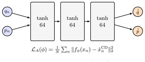
The load-bearing object is the learned scalar Hamiltonian $\hat{H}_\theta(q,p)$ whose symplectic gradient $(\partial_p \hat{H}_\theta, -\partial_q \hat{H}_\theta)$ supplies the vector field; this is what makes the dynamics Hamiltonian by construction. The matched-integrator protocol—identical RK4-generated data, identical central-difference derivative targets, the same Adam settings and seed schedule, and the same RK4 stepper at inference over five seeds—is the control that lets the paper attribute the measured ratios to that architectural prior. The bounded-versus-growing energy-drift signature and the energy-stratified tercile analysis are the diagnostics showing where the prior acts: the standard network's drift grows with horizon and with orbital nonlinearity, while the Hamiltonian network's stays roughly constant.
What would settle it
Train a third architecture under the identical protocol—a scalar-output network whose two-dimensional vector field is produced by multiplying the gradient by a fixed, non-Hamiltonian matrix—and compare long-horizon energy drift; if its drift also saturates near $2\times10^{-4}$, the reported $42\times$/$15.8\times$ ratios would be an effect of scalar parameterization rather than of Hamilton's equations.
Extended reading notes
Core claim
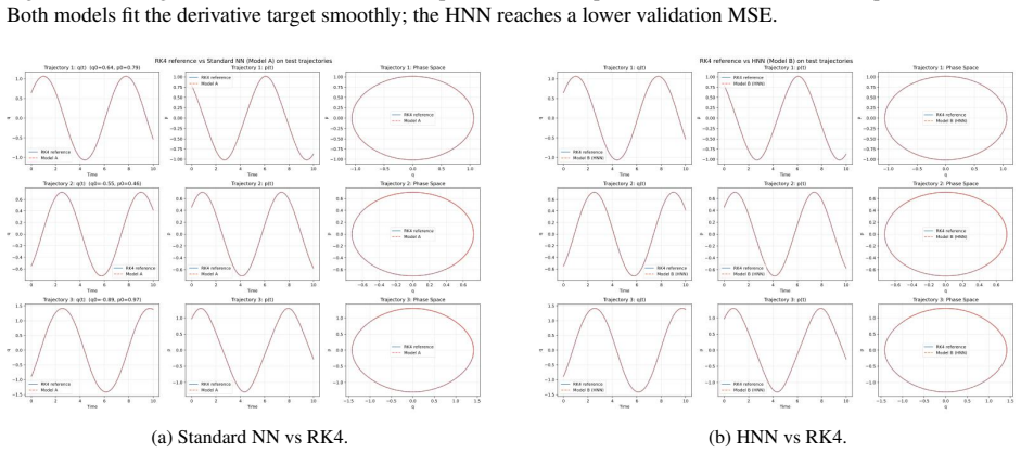
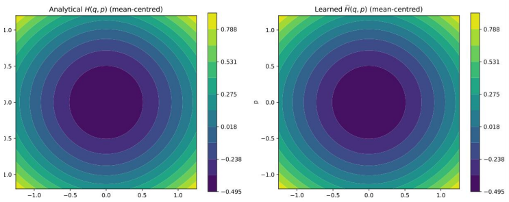
On the paper's own terms, the central discovery is that, once data, supervision, optimization, and inference integration are held fixed, the Hamiltonian parameterization itself accounts for the long-horizon advantage. On the nonlinear pendulum, the learned Hamiltonian's mean maximum energy drift saturates near $2.16\times 10^{-4}$ by $T=5$ and stays flat through $T=100$, while the matched standard network's drift grows monotonically from $2.75\times 10^{-4}$ to $9.08\times 10^{-3}$, a $42\times$ ratio of means at $T=100$; mean trajectory MSE is $15.8\times$ smaller. The learned scalar $\hat{H}_\theta$ matches the analytical pendulum Hamiltonian to RMSE $7.3\times 10^{-5}$ on the training domain, and the saturated drift is the same order as that Hamiltonian-approximation error. In 3D Kepler, the same protocol gives $8.0\pm 1.0\times$ smaller energy drift, $4.2\pm 0.5\times$ smaller angular-momentum drift, and $5.5\pm 0.8\times$ smaller trajectory MSE at $T=10$, even though angular momentum is not in the training loss. The paper also reports a negative diagnostic: an explicit Störmer–Verlet rollout of the learned, non-separable Hamiltonian does not beat HNN+RK4, because the symplecticity guarantee of velocity Verlet only applies to separable Hamiltonians.
Load-bearing premise
The load-bearing premise is that the matched protocol isolates the Hamiltonian prior, because the two models do not start from identical initial weights and the Hamiltonian network has a different output head (a single scalar output, 65 fewer parameters), so part of the gap could in principle come from those remaining differences rather than from Hamilton's equations.
Editorial extensions
If this is right
- At $T=100$ on the pendulum, the Hamiltonian network's energy drift is bounded near $2\times10^{-4}$ while the baseline's grows to $9\times10^{-3}$, so practitioners can trust HNN rollouts over about 16 periods with five-seed-consistent behavior.
- The architectural advantage widens with nonlinearity: from low- to high-energy terciles the baseline's drift grows $4.3\times$ while the HNN's grows only $2.5\times$, so the prior matters most where the vector field is hardest to fit locally.
- The 3D Kepler results show the prior transfers to six-dimensional phase space: energy drift $8.0\times$ smaller, angular-momentum drift $4.2\times$ smaller, and trajectory MSE $5.5\times$ smaller at $T=10$, with angular momentum not explicitly supervised.
- An explicit Störmer–Verlet rollout of a learned non-separable Hamiltonian does not improve over HNN+RK4, implying that structure preservation requires matching the integrator's assumptions (separability or a general symplectic scheme) to the learned model.
- On the 1-DOF pendulum, learned surrogates are slower than RK4 with the analytical vector field, so the computational case for HNNs must rest on many-body scaling, which this paper leaves open.
Reading between the lines
- A testable extension follows from the bounded-drift mechanism: if the benefit comes from scalar parameterization rather than Hamilton's equations, then other scalar-energy architectures (spectral or Gaussian-process Hamiltonians) should reproduce the same saturation under the same protocol.
- The Kepler angular-momentum result is empirical evidence that rotational symmetry is partially captured without explicit equivariance; an explicit rotationally equivariant Hamiltonian parameterization would be the natural test of whether the residual drift closes further.
- The low-data crossover at eight training trajectories is a boundary the paper notes but does not explain; a mechanistic account of when the Hamiltonian prior becomes identifiable would turn this into a practical selection rule.
- Chaotic benchmarks named in the paper, such as Hénon–Heiles or the double pendulum, are the sharpest test of whether bounded drift is a property of integrable systems or of the Hamiltonian prior itself.
Editorial analysis
A structured set of objections, weighed in public.
Referee Report
Summary. This paper evaluates Hamiltonian Neural Networks against a standard feedforward network under a matched-integrator protocol: identical RK4-generated training data, identical central-difference derivative targets, the same optimizer settings and seed schedule, and the same RK4 integrator at inference, with five independent training seeds. On the nonlinear pendulum the HNN is reported to reduce mean maximum energy drift by 42x and mean trajectory MSE by 15.8x at T=100, with bounded rather than growing drift and lower seed-to-seed variance; an energy-stratified analysis shows the gap widening for more nonlinear orbits. A Störmer–Verlet rollout of the learned HNN is analyzed as a diagnostic and does not improve on HNN+RK4. The protocol is then transferred to the three-dimensional Kepler two-body problem, where the HNN shows smaller but consistent advantages in trajectory MSE, energy drift, and angular-momentum drift. The paper also reports computational costs and discusses limitations and future work.
Significance. If the results hold, the paper provides a carefully controlled confirmation of the HNN architectural prior on conservative dynamics. Its strengths include the matched inference integrator, identical supervision targets, multi-seed statistics, the bounded-versus-growing energy-drift diagnostic, the energy-stratified analysis, the honest negative Verlet result, the computational-cost comparison, and a transfer experiment in six-dimensional phase space with an additional conserved quantity. The reported ratios, however, rest on an attribution that is not fully isolated: the HNN differs from the baseline both in its scalar-output/autograd implementation and in the symplectic-gradient structure, and the headline pendulum ratios are sample-mean estimates with large per-seed variance. These issues are fixable with additional control experiments and uncertainty quantification, and they do not undermine the qualitative bounded-drift phenomenon.
major comments (2)
- [§3.3–3.4, §7] The matched-integrator protocol does not fully isolate the Hamiltonian prior from the scalar-output/autograd implementation. Model B differs from Model A in two coupled ways: it has a single scalar output (65 fewer parameters, §3.2) and its vector field is obtained by automatic differentiation of that scalar through Eq. (4), which imposes the symplectic-gradient form. The claim in §7 that 'the only intentional difference is that Model B's vector field is the symplectic gradient of a learned scalar rather than a direct prediction' conflates the architectural prior with its implementation. Because the scalar-output representation and the autograd pipeline could, on their own, change the optimization landscape or the smoothness of the learned field, the 42× and 15.8× ratios are not yet cleanly attributable to Hamiltonian structure. I request an additional control: train a scalar-output network of the same width and depth whose vector field is (∂_p s_θ, ∂_q s_θ) (or another non-Hamiltonian gradient sign) so that the scalar-output/autograd cost is identical but the symplectic structure is absent; if this baseline behaves like Model A, the ratios can be attributed to the Hamiltonian prior, and if it behaves like Model B, the paper's central interpretation needs to be revised.
- [§4.3, Tables 2 and 3] The headline ratios of 15.8× and 42× are ratios of sample means over only five seeds, and Model A's seed-to-seed variance is very large at T=100 (σ/μ > 100% for trajectory MSE and ≈85% for energy drift). No uncertainty interval, paired per-seed ratio, or significance test is reported for these ratios, so the point estimates may be much less stable than the abstract suggests. Please report per-seed ratios (or paired differences on a log scale) and bootstrap confidence intervals for the ratios at each horizon, and state whether the bounded-versus-growing claim is assessed on paired or aggregate statistics. This is important because the quantitative ratios are the paper's central empirical contribution.
minor comments (5)
- [Abstract, Table 1] The abstract and table call Model B 'parameter-matched' although it has 65 fewer parameters than Model A; since 65/8642 is small this is a minor wording issue, but 'near-parameter-matched' or an explicit statement of the difference would be more precise.
- [Table 4] In the low-energy tercile at T=10, Model B's trajectory MSE (4.56±2.65)×10−6 is worse than Model A's (1.24±1.16)×10−6, which is opposite to the energy-drift advantage; the text's claim that the architectural advantage widens with nonlinearity should acknowledge this exception.
- [Table 3] The HNN energy-drift entries for T=10 through T=100 are identical to two significant figures ((2.16±0.90)×10−4); please clarify whether this is rounding of a saturated value and report additional significant digits so readers can verify the saturation claim.
- [§6] The description of initial conditions as 'q0 uniform on spheres of radius r0 ∈ [0.9,1.4]' is ambiguous: specify whether the radius is drawn uniformly and the direction uniformly on the sphere, or whether a different sampling over the shell is used.
- [§3.3] The phrase 'same optimiser state schedule' is imprecise because Adam state tensors have different shapes for the two models; saying 'same optimizer hyperparameters and update schedule' would be accurate.
Circularity Check
No significant circularity: the reported energy-drift and trajectory-error improvements are measured on held-out rollouts of trained models and are not imposed by construction.
full rationale
The paper's central claims are empirical measurements, not derivations that reduce to their inputs. Model B (HNN) is trained only on the derivative-matching loss L_B(theta) = (1/N) sum ||xdot_CD_n - (∂_p H_theta, -∂_q H_theta)||^2, and the headline quantities — maximum absolute energy drift and trajectory MSE at T=100 — are evaluated on held-out test initial conditions after training, over five independent seeds. No fitted parameter or loss term directly encodes energy conservation or long-horizon trajectory accuracy; the bounded-drift behavior emerges from the learned architecture rather than being imposed by the training objective. The matched-integrator control (same RK4 stepper, same data, same derivative targets, same optimizer settings) is actually a strength of the comparison, and the paper explicitly acknowledges the residual confounds, e.g., that HNN has 65 fewer parameters and uses autograd through Eq. (4), and that initial weights are not identical. Acknowledging an imperfect control is not circularity. The Kepler angular-momentum result is likewise an emergent diagnostic: angular momentum does not appear in the training loss, and the paper explicitly cautions that the result is empirical rather than an automatic consequence of the parameterization. The self-citations and references to prior work (Greydanus et al., SympNets, etc.) are used as external context and baselines, not as load-bearing justifications for the measured improvements. The negative result on the HNN+Verlet diagnostic is honestly reported rather than repackaged as a success. No equation in the paper defines a predicted quantity in terms of the fitted parameters in a way that would make the measured outcome true by construction. Hence the appropriate circularity score is 0.
Assumptions & free parameters
free parameters (2)
- Protocol constants (dt, training horizon, architecture width, learning rate, batch size, epochs, seed set) =
dt=1e-2, T_train=10, width=64, lr=1e-3, batch=512, epochs=300, seeds 42-46
- Kepler near-circular initial-condition range =
r0 in [0.9,1.4], p0 perpendicular with speed within ±25% of circular
assumptions (5)
- standard math Hamilton's equations describe the true dynamics of the pendulum and Kepler systems.
- domain assumption RK4 with dt=1e-2 over T=10 provides a sufficiently accurate reference trajectory for training and evaluation.
- domain assumption Central-difference derivative targets approximate true derivatives with O(dt^2) error and do not systematically favor either architecture.
- domain assumption The learned vector fields are smooth enough for fixed-step RK4 inference to be a valid test of the learned dynamics.
- domain assumption The train and test initial-condition distributions cover the regimes over which the conclusions are drawn.
Cite this review
Pith. "Pith review of A matched-integrator evaluation of Hamiltonian neural networks on pendulum and Kepler dynamics." pith.science (2026). https://pith.science/paper/NK2G3TZO
@misc{pith2026260810235,
  author       = {Pith},
  title        = {Pith review of: A matched-integrator evaluation of Hamiltonian neural networks on pendulum and Kepler dynamics},
  year         = {2026},
  howpublished = {\url{https://pith.science/paper/NK2G3TZO}},
  note         = {Machine review of arXiv:2608.10235}
}
read the original abstract
Hamiltonian Neural Networks (HNNs) parameterize conservative dynamics through a learned scalar Hamiltonian, providing an architectural prior that is absent from generic vector-field neural networks. We evaluate this prior under a controlled protocol in which an HNN and a parameter-matched feedforward baseline are trained on the same RK4-generated trajectories, use the same central-difference derivative targets and optimization settings, and are integrated at inference with the same RK4 scheme. Results are reported over five independent training seeds. On the nonlinear pendulum, the HNN reduces mean energy drift by 42-fold and mean trajectory MSE by 15.8-fold at T = 100, approximately 16 pendulum periods. Its energy drift also remains bounded and exhibits substantially lower seed-to-seed variability than the standard-network baseline. An energy-stratified analysis shows that the difference becomes more pronounced as trajectories explore more nonlinear regions of phase space. As an additional diagnostic, we examine an explicit St\"ormer--Verlet-style rollout of the learned HNN. Because the learned Hamiltonian is not constrained to the separable form H(q,p) = T(p) + V(q), the standard symplecticity guarantee of velocity Verlet does not directly apply. We further apply the same matched-integrator protocol to the three-dimensional Kepler two-body problem. The HNN again exhibits lower trajectory, energy, and angular-momentum drift than the parameter-matched baseline. These experiments provide a controlled study of how Hamiltonian parameterization affects long-horizon prediction and physical consistency across two conservative dynamical systems.
Figures


Figures from the paper (7 more)





Reference graph
Works this paper leans on
-
[1]
M. M. Bronstein, J. Bruna, T. Cohen, and P. Veliˇckovi´c. Geometric deep learning: Grids, groups, graphs, geodesics, and gauges. arXiv:2104.13478, 2021
arXiv 2021
-
[2]
R. T. Q. Chen, Y . Rubanova, J. Bettencourt, and D. Duvenaud. Neural Ordinary Differential Equations. In Advances in Neural Information Processing Systems 31, 2018. arXiv:1806.07366
arXiv 2018
-
[3]
M. Cranmer, S. Greydanus, S. Hoyer, P. Battaglia, D. Spergel, and S. Ho. Lagrangian Neural Networks. ICLR 2020 Workshop on Deep Differential Equations. arXiv:2003.04630
arXiv 2020
-
[4]
S. Greydanus, M. Dzamba, and J. Yosinski. Hamiltonian Neural Networks. InAdvances in Neural Information Processing Systems 32, 2019. arXiv:1906.01563
arXiv 2019
- [5]
-
[6]
P. Jin, Z. Zhang, A. Zhu, Y . Tang, and G. E. Karniadakis. SympNets: Intrinsic structure-preserving symplectic networks for identifying Hamiltonian systems.Neural Networks, 132:166–179, 2020. arXiv:2001.03750
arXiv 2020
-
[7]
G. E. Karniadakis, I. G. Kevrekidis, L. Lu, P. Perdikaris, S. Wang, and L. Yang. Physics-informed machine learning.Nature Reviews Physics, 3:422–440, 2021
work page 2021
-
[8]
D. P. Kingma and J. Ba. Adam: A method for stochastic optimization. InInternational Conference on Learning Representations, 2015. arXiv:1412.6980
arXiv 2015
Show all 11 references
-
[9]
Raissi, P
M. Raissi, P. Perdikaris, and G. E. Karniadakis. Physics-informed neural networks: A deep learning framework for solving forward and inverse problems involving nonlinear partial differential equations.Journal of Computational Physics, 378:686–707, 2019
2019
-
[10]
P. Toth, D. J. Rezende, A. Jaegle, S. Racanière, A. Botev, and I. Higgins. Hamiltonian Generative Networks. In International Conference on Learning Representations, 2020. arXiv:1909.13789
2020 arXiv
-
[11]
Y . D. Zhong, B. Dey, and A. Chakraborty. Symplectic ODE-Net: Learning Hamiltonian dynamics with control. In International Conference on Learning Representations, 2020. arXiv:1909.12077. 14
2020 arXiv
Reviewed August 14, 2026 · model on record in the stance chip above.
Discussion (0). Continue with ORCID to comment.