Model reduction for coupled free flow over porous media: a hybrid dimensional pore network model approach

Alexandros Terzis; Guang Yang; Ioannis Zarikos; Kilian Weishaupt; Matthijs de Winter; Rainer Helmig

REVIEW 4 major objections 5 minor 48 references

Model reduction for coupled free flow over porous media: a hybrid dimensional pore network model approach

T0 review · 4 major / 5 minor · reviewed 2026-08-14 · deepseek-v4-flash

Challenge this review Re-run · record.json Download PDF Read on arXiv ↗ Review JSON

Pith's one-line read Two-stage model reduction reproduces a micromodel's pore-scale flow within 6 percent while cutting runtime from hours to minutes.

desk verdict A useful local slip closure for pore-network/free-flow coupling, but a unit inconsistency in the fitted slip coefficient and an overbroad accuracy claim should be fixed before I'd trust the numbers. read the letter →

arxiv 1908.01771 v1 pith:NOH5LMD5 submitted 2019-08-05 physics.comp-ph physics.flu-dyn

Kilian Weishaupt , Alexandros Terzis , Ioannis Zarikos , Guang Yang , Matthijs de Winter , Rainer Helmig This is my paper · ORCID

classification physics.comp-phphysics.flu-dyn

keywords freeflowoverporousmediapore-networkmodelhybrid-dimensionalreductionslipvelocityquasi-3DStokesmicro-PIVmicromodel

verification ladder T0 review T1 audit T2 compute T3 formal

The pith

A machine-rendered reading of the paper's core claim, the machinery that carries it, and where it could break.

The reading

Simulating free flow over a porous medium with fully resolved three-dimensional flow equations costs too much for all but small domains, so the authors ask how far the geometry can be reduced while keeping acceptable accuracy. They first collapse the 3D problem to a quasi-3D plane using a wall-friction drag term, then replace the porous pillar array by an equivalent pore network, leaving only the free-flow channel resolved. The new step is a per-throat slip condition at openings between channel and network, with a slip coefficient $\beta_{\text{throat}}$ fitted numerically on isolated throat geometries and extrapolated by a power-law fit. Against the fully resolved reference, the coupled model reproduces integrated throat fluxes within about 6%, keeps velocity and pressure relative errors near $10^{-2}$ and $10^{-4}$, and cuts runtime from roughly five hours on 30 cores to under five minutes on one core. The authors' claim is that this simple, local modification makes hybrid-dimensional models accurate enough for larger coupled free-flow/porous problems.

What carries the argument

The carrying mechanism is a local slip coupling condition at each pore throat that opens onto the free-flow channel. It prescribes the tangential free-flow velocity at the opening as $$v_{\text{slip},i} = \frac{1}{\beta_{\text{throat}}}\big[(-\mu(\nabla\mathbf{v}+\nabla\mathbf{v}^T)\mathbf{n})\cdot\mathbf{t}_i\big]^{\text{FF}} + [\mathbf{v}]^{\text{PNM}}\cdot\mathbf{t}_i,$$ with $\beta_{\text{throat}}$ determined numerically from an isolated orthogonal-throat problem; this replaces the earlier condition, which yielded no slip whenever the throat was perpendicular to the interface. The rest of the reduction chain consists of the quasi-3D Stokes model with drag term $-(8\mu/h^2)\mathbf{v}_{2D}$, pore-network throat conductances $k_{ij}$ obtained by numerical upscaling on a reduced equivalent pillar structure, and a fully monolithic (single-system) coupling that enforces mass and pressure continuity at the interface. The empirical power-law fit $\beta_{\text{throat}}\approx 4.531\,w_{\text{throat}}^{-1.067}$ (units of $\mathrm{m}^{-1}$, $R^2=0.999$) extends the calibrated coefficient to other throat widths without re-solving the calibration problem; without wall friction the fit is $\approx 7.680\,w_{\text{throat}}^{-1.019}$.

What would settle it

Take the same micromodel with the pore openings tilted by 45 degrees, run the coupled model with the coefficient fitted on perpendicular openings, and compare the velocity immediately above each opening with a fully resolved 3D simulation; if the integrated throat fluxes leave the 6 percent agreement band, the single-coefficient transferability fails.

Watch

Extended reading notes

Core claim

The central claim is that a hybrid-dimensional model can stand in for a fully resolved three-dimensional simulation of a micromodel with a free-flow channel over a porous pillar array, as long as the pore-network coupling includes slip at the throat mouths. The earlier coupling forced the tangential component of the pore-throat velocity onto the free-flow boundary, which degenerates to no slip for throats meeting the interface at right angles; this paper replaces that with continuity of tangential stress, balancing the free-flow shear against a per-throat slip coefficient $\beta_{\text{throat}}$ fitted on a simplified single-throat geometry. For the full micromodel, the coupled model's integrated fluxes through all 81 interface throats fall within about 6% of the 3D reference, its velocity and pressure fields deviate from the quasi-3D reference by relative errors of $9.5\times10^{-3}$ and $3.7\times10^{-4}$, and the runtime is about 5 minutes on one core versus about 5 hours on 30 cores. Including the slip term improves the isolated orthogonal-throat velocity error by a factor of 9 over the no-slip coupling, with no added runtime; the authors also show the improvement persists, but is weaker, for an inclined throat with inflow.

Load-bearing premise

The whole result depends on a single fitted number—how strongly the fluid slips at a pore opening—being good enough for every opening in the whole porous structure, even though it was calibrated on one simple opening with no sideways current.

Editorial extensions

If this is right

The slip condition is local and adds no runtime, so the same coupling can be extended to other free-flow/pore-network geometries of this type; in the isolated orthogonal-throat test it reduces the velocity error by a factor of 9 compared with the no-slip coupling.
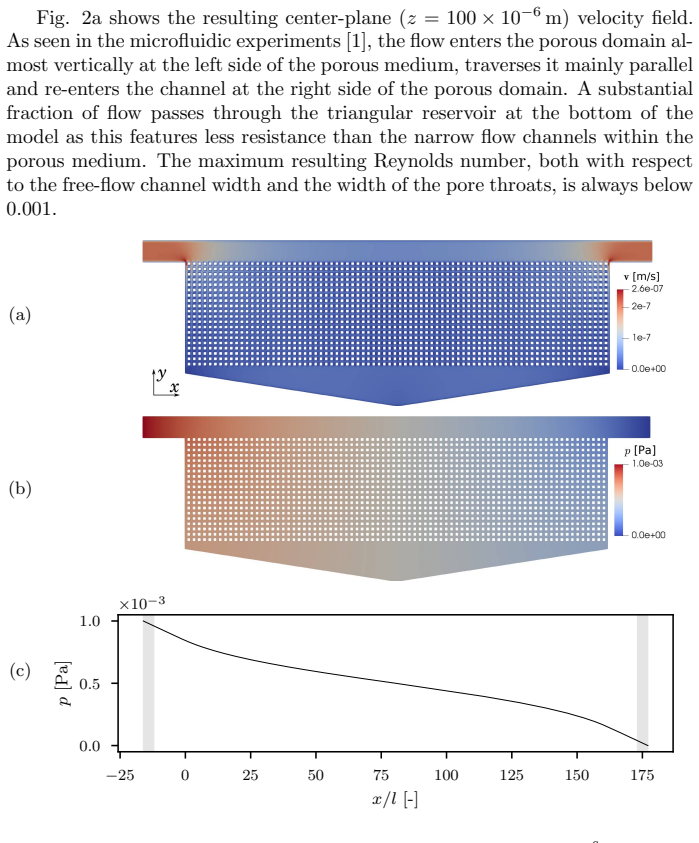
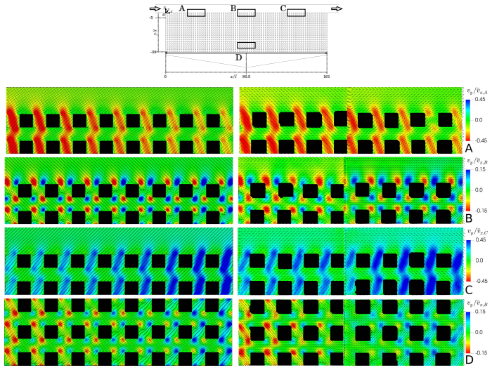
Integrated interface quantities are more reliable than local ones: the coupled model over-predicts some near-throat vertical velocity peaks by up to 80%, yet the total flux through each interface throat stays within about 6% of the 3D reference.
The power-law fit $\beta_{\text{throat}}\approx 4.531\,w_{\text{throat}}^{-1.067}$ lets the calibrated slip coefficient be reused for other throat widths without re-solving the calibration problem, at least for perpendicular, no-inflow throat configurations.
The reduction shortens a full-array micromodel simulation from about five hours on 30 cores to under five minutes on one core, and the coupled model is 2.3 times faster than the quasi-3D model alone, making parameter sweeps and design optimization practical.

Reading between the lines

Editorial extensions of the paper, not claims the author makes directly.

Editorial inference: the single-coefficient calibration is the fragile link; the paper's own inclined-throat test shows $\beta_{\text{throat}}$ dropping from $84550$ to $28001$ at the same $100\,\mu\mathrm{m}$ width, so applying the orthogonal no-inflow coefficient to a network with inclined or cross-flowing throats is a direct test of where the 6% flux agreement would break down.
Editorial inference: because the slip coefficient is extracted from the same quasi-3D model class used as the validation reference, the comparison does not independently confirm the slip law against true 3D flow; high-resolution velocity measurement directly at a throat mouth would close that gap.
Editorial inference: local errors concentrate at throat edges and cancel in integrated fluxes, so interfacial quantities that respond to local shear—surface deposition, dissolution, or wall reactions—should be treated with caution even where total mass exchange is accurate.
Editorial inference: generalizing $\beta_{\text{throat}}$ to depend on throat orientation and inflow strength, or replacing the scalar fit with a local analytical slip expression, is the natural next step toward realistic geometries where interface throats are rarely perfectly perpendicular.

Share X Bluesky LinkedIn Reddit HN

Signed reviews

No signed human review yet.

Editorial analysis

A structured set of objections, weighed in public.

Desk editor's note, referee report, and a circularity audit.

Desk Editor's Note

read the letter

The genuinely new thing here is the local, per-throat slip condition at pore-throat/free-flow intersections. It fixes the no-slip artifact of the authors' earlier model for orthogonal throats. The implementation is clean, the slip term clearly improves the velocity field (a factor of 9 reduction in the isolated-throat velocity error), and the runtime speedup is credible.

The soft spots, in order of severity. First, there is a dimensional problem in the definition of beta_throat. Eq (3.16)/(3.18) require beta to have units Pa s/m, but Eq (4.4) and all tabulated values give 1/m. Either the stress balance should use the shear rate without the viscosity, or the fitted beta is intended to be multiplied by mu. The paper does not say which convention the DuMux implementation uses, so the central quantitative claims are not reproducible until this is resolved. I cannot assign a physical meaning to the fitted value as written. This is the most fundamental issue.

Second, the abstract's 'less than 10%' is too broad. Fig 19 shows local vertical-velocity discrepancies up to 80% at the edges of throat openings. The global errors are small and the mass exchange is captured, but the claim needs to be qualified to integrated or global quantities.

Third, the calibration/validation loop is partly circular. beta_throat and the conductances kij are fitted to quasi-3D reference solutions, and then the coupled model is validated against the same quasi-3D model class. The comparison with 3D OpenFOAM throat fluxes in Fig 20 helps, but the coupled velocity field is never checked against the full 3D simulation or the experiment. The transferability of beta from an isolated orthogonal throat to the 81-throat network is fragile—the inclined-throat test shows beta changes by a factor of 3 for the same width—though in this geometry all interface throats are orthogonal, so it is an acceptable assumption for the main test case.

None of this kills the paper. The central idea is sound, the numerics are careful, and the authors are honest about limitations. There is real value for people building hybrid-dimensional models of microfluidic and porous-media flows. It deserves peer review, but I would send it back with a request to fix the units, qualify the accuracy claims, and ideally release code and data.

Referee Report

4 major / 5 minor

Summary. The paper proposes a two-stage model reduction for steady creeping flow in a micromodel consisting of a free-flow channel over a regular porous medium. The authors first build a fully resolved 3D OpenFOAM Stokes model, validate it against high-resolution micro-PIV data, and then reduce it to a quasi-3D 2D model with a wall-friction closure. In the second stage, the porous part is replaced by a pore-network model, coupled monolithically to the quasi-3D free-flow model. The new element is a slip boundary condition at each pore-throat intersection with the free-flow interface, parameterized by a per-throat slip coefficient β_throat that is calibrated from isolated quasi-3D reference solutions. The reported results include a global relative velocity error of 9.49e-3 and a pressure error of 3.72e-4 for the coupled model against the quasi-3D solution, integral throat fluxes within about 6% of the 3D simulation, and a runtime reduction from roughly five hours on 30 cores to under five minutes on a single core.

Significance. If the quantitative claims can be made fully reproducible, this is a useful contribution: the per-throat slip closure removes the artificial no-slip constraint of the earlier model, improves the velocity error by a factor of about 9 in the single-throat test, and retains pore-scale detail at a small fraction of the cost of the resolved simulation. The fact that the 3D reference model is compared with micro-PIV experiments gives the reduction chain a credible anchor. The paper is also reasonably candid about limitations, including the degraded behavior for inclined throats and the large local deviations near the edges of throat openings in Fig. 19. However, the central error claims currently rest on a slip coefficient whose definition is dimensionally inconsistent between the model equations and the calibration formula, and the coupled model is validated against the same quasi-3D model class used for calibration. These issues must be resolved before the paper can be considered ready.

major comments (4)

[Sec. 3.3, Eqs. (3.16)/(3.18); Sec. 4.3, Eq. (4.4); Table 1] The slip coefficient is dimensionally inconsistent. In Eq. (3.16), the left-hand side [(-µ(∇v+∇v^T)·n)·t]_FF is a shear stress with units Pa, so β_throat in Eq. (3.18) must have units Pa·s/m for v_slip to be a velocity. However, Eq. (4.4) defines β_throat as a shear rate divided by a velocity, which has units 1/m, and Table 1 lists β in 1/m. Unless the DuMux implementation multiplies the fitted quantity by the viscosity (which is nowhere stated), the tabulated values cannot be substituted into Eq. (3.18). The central quantitative claims — relative velocity error 9.49e-3, pressure error 3.72e-4, and the abstract's '<10%' statement — all depend on this parameter. The authors must state the convention used in the implementation and make the reported numbers consistent with that convention before the results can be reproduced or checked.
[Abstract; Sec. 4.4, Fig. 19] The abstract's claim that the coupled model deviates by less than 10% from the other two model concepts is not supported as stated. The global relative L2 errors reported in Sec. 4.4 are 9.49e-3 for velocity and 3.72e-4 for pressure, but Fig. 19 shows local vertical-velocity discrepancies of up to 80% at the edges of the throat openings. The paper should explicitly state that the 10% figure refers to global norms, quantify the local deviations in the abstract, and discuss their practical consequence for quantities such as interfacial mass exchange, as is partially done around Fig. 20.
[Secs. 4.3 and 4.4] The validation loop is partially circular. The throat conductances kij are obtained by numerical upscaling on a quasi-3D pillar structure, and β_throat is fitted from isolated quasi-3D reference solutions; the full coupled model is then compared against the quasi-3D solution of the same micromodel. The reported velocity and pressure errors are therefore consistency checks of the reduction chain, not independent tests against the 3D reference or the experimental data. Direct comparison with the 3D OpenFOAM fields is provided only for integrated throat fluxes in Fig. 20. The paper should either add a direct comparison of the coupled model's velocity/pressure fields with the 3D solution or explicitly restrict the claims to quasi-3D consistency.
[Sec. 4.3, Figs. 12 and 14] The transferability of a single β_throat value to the full 81-throat network is fragile and is not quantified. The calibration set gives β_throat varying by roughly a factor of 9 over throat widths from 50 to 400 µm, and the inclined-throat test changes β from 84550 to 28001 1/m for the same 100 µm width. The full coupled model uses a single value β = 33000 1/m from the power-law fit. The text states that the re-evaluated β gives 'very similar results,' but no results are shown to support this. A sensitivity study of the coupled model's global errors with respect to β_throat is needed to justify the single-parameter closure and to determine how much of the 80% local deviation in Fig. 19 is controlled by this parameter.

minor comments (5)

[Sec. 4, first paragraph] The term 'βthoat' is a typo and should read 'βthroat'.
[Sec. 3.3, Eq. (3.9)] The text near Eq. (3.9) contains 'Qis' and an incomplete definition; it should read 'Qij' with a complete sentence defining the discrete flow rate.
[Sec. 4.3] The terminology switches between 'conductance' and 'resistance' for kij; the authors should use one term consistently and state the units in the text.
[Fig. 12] The power-law fits should state the units of the prefactor and of wthroat, and should be reconciled with the stated unit of β; currently the plotted values inherit the dimensional ambiguity of Eq. (4.4).
[Sec. 5] The CPU-time comparison is appropriately caveated in Sec. 5, but the abstract should mention that the 3D solver is transient and parallelized while the reduced models are stationary and serial, so the speedup is not a direct wall-clock comparison.

Circularity Check

1 steps flagged · score 5.0 of 10

The slip coefficient β_throat is calibrated on the quasi-3D reference and then re-used to 'predict' the same reference setups; the full micromodel comparison is only partially calibrated, with independent 3D flux checks.

fitted input called prediction [Sec. 4.3, Eq. (4.4), Table 1]
"The slip velocities and velocity gradients at the interface between pore throat and free flow (corresponding to y/l = 0) are then extracted, averaged and used to approximate the slip coefficient: βthroat≈⟨∂vx/∂y+∂vy/∂x⟩/⟨vx⟩ ... The resulting factors are given in the last column of Tab. 1 and then used for recalculating the given setups using the coupled model, i.e, replacing the small cavity by a single one-dimensional pore throat of the same width and length."

βthroat is obtained from the quasi-3D reference solution of exactly the isolated orthogonal-throat geometry: Eq. (4.4) is the ratio of the averaged shear rate to the averaged interface velocity. Eq. (3.18) then uses this same coefficient to set the coupled model's interface slip velocity, so for the orthogonal no-inflow calibration case the coupled model is forced to match the reference's average slip velocity. The 'virtually identical' velocity profiles in Table 1 are therefore a consistency check of the calibration, not an independent prediction. The full micromodel run is less directly circular (β=33,000 m^-1 is interpolated and the 81-throat network is a different problem, and Fig. 20 checks against 3D OpenFOAM), but it inherits the same quasi-3D calibration source.

full rationale

The paper's reduction chain is mostly transparent: a fully resolved 3D Stokes model is validated against micro-PIV data, the quasi-3D model with wall drag is compared with that 3D reference, and the coupled pore-network model is then compared with both quasi-3D and 3D results. The main circularity is confined to the calibration of the new slip coefficient. βthroat is extracted from the averaged shear rate and velocity of a quasi-3D reference solution and then inserted back into the coupled model for the same isolated-throat setups; the close agreement shown in Table 1 is therefore a back-calculation rather than an independent predictive test. The full 81-throat micromodel run is not algebraically identical to the fitting input: β is extrapolated to 240 µm by a power-law fit, the conductances kij come from a separate reduced-structure upscaling taken from the authors' prior work [2], and the integrated throat fluxes are also compared with the independent 3D OpenFOAM solution in Fig. 20, with about 6% deviation. That independent 3D comparison prevents the central claim from collapsing entirely into a fit. The paper itself reports a transferability limitation: re-evaluating β for the inclined-throat setup changes the value from 84550 to 28001, yet the orthogonal value is still used; this weakens the claimed generality but is a limitation rather than circularity. Separately, Eqs. (3.16)/(3.18) and (4.4) appear dimensionally inconsistent (Pa vs m^-1 units for β), which is a correctness/reproducibility concern, not a circularity finding. Overall, the new slip-closure validation is partially circular, while the full-model claim retains meaningful independent content, so a moderate score is appropriate.

Assumptions & free parameters 2 free parameters · 6 assumptions · 0 invented entities

The central results rest on two calibrated closures (beta_throat and kij) and on several modeling assumptions that restrict validity to steady creeping single-phase flow with primarily orthogonal pore-throat intersections. No new physical entities are postulated.

free parameters (2)

beta_throat (throat slip coefficient) = 33000 1/m for w=240 um (power-law fit 4.531 w^-1.067, R^2=0.999; fitted values 176416, 84550, 39924, 19087 1/m for…
Introduced in Eqs. (3.16)-(3.18) as a per-throat closure coefficient and determined numerically in Sec. 4.3 from averaged shear rate and velocity of a simplified quasi-3D reference simulation via Eq. (4.4). The accuracy of the slip coupling depends on this calibrated value.
k_ij,t and k_1/2,i (throat and pore-body conductance factors) = k_ij,t = 3.05e-10 m3/(sPa), k_1/2,i = k_1/2,j = 8.47e-10 m3/(sPa)
Pore-throat conductance parameters in Eqs. (3.10) and (4.3), obtained by numerical upscaling of pressure-drop boundary value problems on a reduced pillar structure (appendix of [2]). They set the porous-medium flow resistance in the coupled model.

assumptions (6)

domain assumption Flow is steady, incompressible, creeping (Re<1), isothermal, and gravity is neglected with fixed fluid properties.
Sec. 3 states these assumptions and restricts the method to creeping single-phase Stokes flow.
domain assumption The velocity profile in the omitted z-direction is parabolic, so the Hele-Shaw drag term -(8 mu / h^2) v_2D captures wall shear.
Sec. 3.2, Eq. (3.4). This is the quasi-3D reduction premise; the authors note the aspect ratio in pore throats (0.83) makes it less accurate there.
domain assumption Pore-network throat flux is linear in pressure difference and pore-body pressure has the same physical meaning as Stokes pressure, allowing pressure continuity at the interface.
Sec. 3.3, Eqs. (3.10)-(3.12), based on a 1D Stokes derivation [35] and the numerical upscaling of kij from [2].
ad hoc to paper Tangential momentum transfer across each pore-throat intersection can be represented by a constant per-throat slip coefficient beta_throat via Eq. (3.16).
Sec. 3.3, Eqs. (3.16)-(3.18). This parametrization is the paper's novel closure and is not derived from first principles.
ad hoc to paper beta_throat evaluated for a single isolated orthogonal throat without through-flow transfers to the full 81-throat micromodel, including inclined throats with inflow.
Sec. 4.3-4.4. The authors acknowledge limitations for the inclined case (beta=28001 vs 84550) but still use the orthogonal value in the full model.
domain assumption Numerically upscaled conductance factors from a reduced 2D pillar structure are valid for the full micromodel pore network.
Sec. 4.3, Eq. (4.3), relies on the appendix of [2] for the upscaling procedure.

how reviews work

0 comments

Cite this review

Pith. "Pith review of Model reduction for coupled free flow over porous media: a hybrid dimensional pore network model approach." pith.science (2026). https://pith.science/paper/NOH5LMD5

@misc{pith2026190801771,
  author       = {Pith},
  title        = {Pith review of: Model reduction for coupled free flow over porous media: a hybrid dimensional pore network model approach},
  year         = {2026},
  howpublished = {\url{https://pith.science/paper/NOH5LMD5}},
  note         = {Machine review of arXiv:1908.01771}
}

read the original abstract

Modeling coupled systems of free flow adjacent to a porous medium by means of fully resolved Navier-Stokes equations is limited by the immense computational cost and is thus only feasible for relatively small domains. Model reduction allows to decrease a model's complexity while maintaining an acceptable degree of accuracy. Starting from a fully resolved three-dimensional numerical model, which is compared to high-resolution micro-PIV experimental data obtained from a previous study (Terzis et al.,2019), we perform a two-fold model reduction: first, a quasi-3D model incorporating a wall friction term is successfully compared to the fully resolved model. Second, we employ a pore-network model to account for the porous part of the domain and couple it to the quasi-3D model which still resolves the free-flow part of the domain (Weishaupt et al., 2019). We have extended this coupling approach here to include slip velocities at the pore throats intersecting with the free-flow domain. The proposed method is simple, accurate and comes at no additional run-time penalty. The coupled model deviates by less than 10 % from the other two model concepts. Several hours of run-time was required for the three-dimensional model compared to eleven and five minutes necessary for the quasi-3D and coupled model which highlights the benefits of model reduction.

Figures

Figures reproduced from arXiv: 1908.01771 by the authors.

**Figure 2.** Center-plane velocity (a) and and pressure (b) field ( [PITH_FULL_IMAGE:figures/full_fig_p009_2.png] view at source ↗

**Figure 3.** Stream-wise velocity profiles at the left inlet of the free flow channel over the channel [PITH_FULL_IMAGE:figures/full_fig_p010_3.png] view at source ↗

Figures from the paper (18 more)

**Figure 4.** Figure 4: Comparison of flow fields obtained by numerical simulation with OpenFoam (left [PITH_FULL_IMAGE:figures/full_fig_p011_4.png]

**Figure 5.** Figure 5: Left (a): Comparison of averaged velocity profiles (75 [PITH_FULL_IMAGE:figures/full_fig_p012_5.png]

**Figure 6.** Figure 6: Comparison of the flow angles θ close to the interface between free flow and porous medium at y/l = 0.5 (top) and y/l = 0.1 (bottom) for the simulation and the experiment.The original data of [1] were used. In summary, we find that the numerical model is able to reprod…

**Figure 7.** Figure 7: Two-dimensional velocity field (v2D) obtained by the quasi-3D model corresponding to the center plane (z = 100 × 10−6 m) of the 3D model. The quasi-3D model captures the main features of the flow accurately when compared to Fig. 2a. For a quantitative comparison, [PIT…

**Figure 8.** Figure 8: Difference between the 3D and quasi-3D velocity fields. [PITH_FULL_IMAGE:figures/full_fig_p014_8.png]

**Figure 9.** Figure 9: depicts the profiles of p and vx along the free-flow channel’s central axis in the x-direction for both the 3D and quasi-3D simulation. All values are normalized by the maximum values of the 3D simulation. The pressure curves are virtually identical and, as stated earl…

**Figure 10.** Figure 10: Left (a): Velocity profiles vx over y at y/l = 80.5 for the 3D and quasi-3D model. Right (b): Velocity profile at the inlet of the free-flow channel and corresponding analytical solution [41]. For comparison, also a parabolic flow profile, neglecting the friction of t…

**Figure 11.** Figure 11: Normalized vy at the interface in stream-wise direction (y/l = 0) for the 3D and quasi-3D model. 4.3. Numerical determination of the conductance factor kij and the slip coefficient βthroat In the final step of model reduction, a pore-network model is used to account …

**Figure 12.** Figure 12: Plot of βthroat over wthroat for a case considering the bottom and wall friction (h = 200 µm) and a case neglecting this influence [PITH_FULL_IMAGE:figures/full_fig_p021_12.png]

**Figure 13.** Figure 13: Close-up of the interface region (see gray inlay) for a vertical throat with [PITH_FULL_IMAGE:figures/full_fig_p022_13.png]

**Figure 14.** Figure 14: Close-up of the interface region (see gray inlay) for an inclined throat with [PITH_FULL_IMAGE:figures/full_fig_p023_14.png]

**Figure 15.** Figure 15: Comparison of the shear rates at the interface for the orthogonal setup (Fig. 13 [PITH_FULL_IMAGE:figures/full_fig_p023_15.png]

**Figure 16.** Figure 16: Two-dimensional velocity field (v2D, top) and pressure field (bottom) obtained by the coupled model corresponding to the center plane (z = 100 × 10−6 m) of the 3D model. The one-dimensional throat elements of the pore-network model have been extruded for visualizatio…

**Figure 17.** Figure 17: Close-up of the interface region at the central throat ( [PITH_FULL_IMAGE:figures/full_fig_p026_17.png]

**Figure 18.** Figure 18: Close-up of the interface region at the two leftmost throats (0 [PITH_FULL_IMAGE:figures/full_fig_p026_18.png]

**Figure 19.** Figure 19: Normalized vy at the interface in stream-wise direction (y/l = 0) for the quasi-3D and the coupled model. Here, the total volumetric flow through each throat at the interface is shown, as evaluated by Eqs. (3.3) and (3.8). The throats are label from left to right from…

**Figure 20.** Figure 20: Discrete volumetric flow rates at all throats intersecting with the interface for all [PITH_FULL_IMAGE:figures/full_fig_p028_20.png]

**Figure 21.** Figure 21: Velocity profiles vx over y at x/l = 80.5 and discrete volumetric flow rates at x/l = 79.5 for all numerical models, normalized by the maximum values of OpenFoam.The coupled model only features continuous velocities in the free-flow channel and the triangular region. …

Discussion (0). Continue with ORCID to comment.

Reference graph

Works this paper leans on

48 extracted references · 44 canonical work pages

[1]

Terzis, I

A. Terzis, I. Zarikos, K. Weishaupt, G. Yang, X. Chu, R. Helmig, B. Weigand, Microscopic velocity ﬁeld measurements inside a regular porous medium adjacent to a low reynolds number channel ﬂow, Physics of Fluids 31 (4) (2019) 042001 (Apr. 2019). doi:10.1063/1.5092169. URL https://doi.org/10.1063/1.5092169

work page doi:10.1063/1.5092169 2019
[2]

Weishaupt, V

K. Weishaupt, V. Joekar-Niasar, R. Helmig, An eﬃcient coupling of free ﬂow and porous media ﬂow using the pore-network modeling approach, Journal of Computational Physics: X 1 (2019) 100011 (Jan. 2019). doi: 10.1016/j.jcpx.2019.100011. URL https://doi.org/10.1016/j.jcpx.2019.100011

arXiv 2019
[3]

Vanderborght, T

J. Vanderborght, T. Fetzer, K. Mosthaf, K. M. Smits, R. Helmig, Heat and water transport in soils and across the soil-atmosphere interface: 1. Theory and diﬀerent model concepts, Water Resources Research 53 (2) (2017) 1057–1079 (2017)

work page 2017
[4]

V. P. Chauhan, T. Stylianopoulos, Y. Boucher, R. K. Jain, De- livery of Molecular and Nanoscale Medicine to Tumors: Transport Barriers and Strategies, Annual Review of Chemical and Biomolec- ular Engineering 2 (1) (2011) 281–298 (Jul. 2011). doi:10.1146/ annurev-chembioeng-061010-114300 . URL https://doi.org/10.1146/annurev-chembioeng-061010-114300

work page doi:10.1146/annurev-chembioeng-061010-114300 2011
[5]

Verboven, D

P. Verboven, D. Flick, B. Nicola¨ ı, G. Alvarez, Modelling transport phenom- ena in refrigerated food bulks, packages and stacks: basics and advances, International Journal of Refrigeration 29 (6) (2006) 985–997 (2006)

work page 2006
[6]

Gurau, J

V. Gurau, J. A. Mann, A critical overview of computational ﬂuid dynamics multiphase models for proton exchange membrane fuel cells, SIAM Journal on Applied Mathematics 70 (2) (2009) 410–454 (2009)

work page 2009
[7]

G. Yang, B. Weigand, A. Terzis, K. Weishaupt, R. Helmig, Numerical Simulation of Turbulent Flow and Heat Transfer in a Three-Dimensional Channel Coupled with Flow Through Porous Structures, Transport in Porous Media 122 (1) (2018) 145–167 (Jan. 2018). doi:10.1007/ s11242-017-0995-9 . URL https://doi.org/10.1007/s11242-017-0995-9

work page doi:10.1007/s11242-017-0995-9 2018
[8]

Whitaker, The method of volume averaging, Kluwer Academic, 1999 (1999)

S. Whitaker, The method of volume averaging, Kluwer Academic, 1999 (1999)

work page 1999

Show all 48 references

[9]

H. C. Brinkman, A calculation of the viscous force exerted by a ﬂowing ﬂuid on a dense swarm of particles, Applied Scientiﬁc Research 1 (1) (1949) 27–34 (1949). 31

1949
[10]

J. A. Ochoa-Tapia, S. Whitaker, Momentum transfer at the boundary be- tween a porous medium and a homogeneous ﬂuid—I. Theoretical devel- opment, International Journal of Heat and Mass Transfer 38 (14) (1995) 2635–2646 (1995)

1995
[11]

W. J. Layton, F. Schieweck, I. Yotov, Coupling ﬂuid ﬂow with porous media ﬂow, SIAM Journal on Numerical Analysis 40 (6) (2002) 2195–2218 (2002)

2002
[12]

Jamet, M

D. Jamet, M. Chandesris, B. Goyeau, On the equivalence of the discontinu- ous one-and two-domain approaches for the modeling of transport phenom- ena at a ﬂuid/porous interface, Transport in Porous Media 78 (3) (2009) 403–418 (2009)

2009
[13]

Mosthaf, K

K. Mosthaf, K. Baber, B. Flemisch, R. Helmig, A. Leijnse, I. Rybak, B. Wohlmuth, A coupling concept for two-phase compositional porous- medium and single-phase compositional free ﬂow, Water Resour. Res 47 (10) (2011)

2011
[14]

S. M. Hassanizadeh, W. G. Gray, Derivation of conditions describing trans- port across zones of reduced dynamics within multiphase systems, Water Resour. Res 25 (3) (1989) 529–539 (1989)

1989
[15]

Shahraeeni, P

E. Shahraeeni, P. Lehmann, D. Or, Coupling of evaporative ﬂuxes from drying porous surfaces with air boundary layer: Characteristics of evapo- ration from discrete pores, Water Resour. Res 48 (9) (2012)

2012
[16]

T. D. Scheibe, E. M. Murphy, X. Chen, A. K. Rice, K. C. Carroll, B. J. Palmer, A. M. Tartakovsky, I. Battiato, B. D. Wood, An analysis platform for multiscale hydrogeologic modeling with emphasis on hybrid multiscale methods, Groundwater 53 (1) (2015) 38–56 (2015)

2015
[17]

Oostrom, Y

M. Oostrom, Y. Mehmani, P. Romero-Gomez, Y. Tang, H. Liu, H. Yoon, Q. Kang, V. Joekar-Niasar, M. Balhoﬀ, T. Dewers, et al., Pore-scale and continuum simulations of solute transport micromodel benchmark experi- ments, Computational Geosciences 20 (4) (2016) 857–879 (2016)

2016
[18]

M. T. Balhoﬀ, K. E. Thompson, M. Hjortsø, Coupling pore-scale networks to continuum-scale models of porous media, Computers & Geosciences 33 (3) (2007) 393–410 (2007)

2007
[19]

Arbogast, G

T. Arbogast, G. Pencheva, M. F. Wheeler, I. Yotov, A multiscale mor- tar mixed ﬁnite element method, Multiscale Modeling & Simulation 6 (1) (2007) 319–346 (2007)

2007
[20]

Mehmani, M

Y. Mehmani, M. T. Balhoﬀ, Bridging from pore to continuum: A hybrid mortar domain decomposition framework for subsurface ﬂow and transport, Multiscale Modeling & Simulation 12 (2) (2014) 667–693 (2014). 32

2014
[21]

Beyhaghi, Z

S. Beyhaghi, Z. Xu, K. M. Pillai, Achieving the Inside–Outside Coupling During Network Simulation of Isothermal Drying of a Porous Medium in a Turbulent Flow, Transport in Porous Media 114 (3) (2016) 823–842 (2016)

2016
[22]

OpenFoam version 1806, https://www.openfoam.com/, accessed: 2019- 08-05

2019
[23]

E. G. Flekkøy, U. Oxaal, J. Feder, T. Jøssang, Hydrodynamic dispersion at stagnation points: Simulations and experiments, Physical Review E 52 (5) (1995) 4952–4962 (Nov. 1995). doi:10.1103/physreve.52.4952. URL https://doi.org/10.1103/physreve.52.4952

1995 doi
[24]

Venturoli, E

M. Venturoli, E. S. Boek, Two-dimensional lattice-boltzmann simulations of single phase ﬂow in a pseudo two-dimensional micromodel, Physica A: Statistical Mechanics and its Applications 362 (1) (2006) 23–29 (Mar. 2006). doi:10.1016/j.physa.2005.09.006. URL https://doi.org/10.1...

2006 doi
[25]

Laleian, A

A. Laleian, A. Valocchi, C. Werth, An incompressible, depth-averaged lat- tice boltzmann method for liquid ﬂow in microﬂuidic devices with vari- able aperture, Computation 3 (4) (2015) 600–615 (Nov. 2015). doi: 10.3390/computation3040600. URL https://doi.org/10.3390/computation3040600

2015 doi
[26]

P. Kunz, I. M. Zarikos, N. K. Karadimitriou, M. Huber, U. Nieken, S. M. Hassanizadeh, Study of multi-phase ﬂow in porous media: Com- parison of SPH simulations with micro-model experiments, Transport in Porous Media 114 (2) (2015) 581–600 (Nov. 2015). doi:10.1007/ s11242-015-0...

2015 doi
[27]

Flemisch, M

B. Flemisch, M. Darcis, K. Erbertseder, B. Faigle, A. Lauser, K. Mosthaf, S. M¨ uthing, P. Nuske, A. Tatomir, M. Wolﬀ, et al., DuMux: DUNE for multi-{phase, component, scale, physics,. . .} ﬂow and transport in porous media, Advances in Water Resources 34 (9) (2011) 1102–1112 (2011)

2011
[28]

T. Koch, D. Gl¨ aser, K. Weishaupt, S. Ackermann, M. Beck, B. Becker, S. Burbulla, H. Class, E. Coltman, T. Fetzer, B. Flemisch, C. Gr¨ uninger, K. Heck, J. Hommel, T. Kurz, M. Lipp, F. Mohammadi, M. Schneider, G. Seitz, S. Scholz, F. Weinhardt, Dumux 3.0.0 (Dec. 2018). doi:10...

2018
[29]

Bastian, M

P. Bastian, M. Blatt, A. Dedner, C. Engwer, R. Kl¨ ofkorn, M. Ohlberger, O. Sander, A generic grid interface for parallel and adaptive scientiﬁc com- puting. Part I: Abstract framework, Computing 82 (2) (2008) 103–119 (2008). 33

2008
[30]

Bastian, M

P. Bastian, M. Blatt, A. Dedner, C. Engwer, R. Kl¨ ofkorn, R. Kornhuber, M. Ohlberger, O. Sander, A generic grid interface for parallel and adaptive scientiﬁc computing. Part II: Implementation and tests in DUNE, Com- puting 82 (2-3) (2008) 121–138 (2008)

2008
[31]

F. H. Harlow, J. E. Welch, Numerical calculation of time-dependent viscous incompressible ﬂow of ﬂuid with free surface, The Physics of Fluids 8 (12) (1965) 2182–2189 (1965)

1965
[32]

H. K. Versteeg, W. Malalasekera, An introduction to computational ﬂuid dynamics: the ﬁnite volume method, Pearson Education, 2007 (2007)

2007
[33]

T. A. Davis, Algorithm 832: UMFPACK V4.3 - an unsymmetric- pattern multifrontal method, ACM Transactions on Mathematical Software (TOMS) 30 (2) (2004) 196–199 (2004)

2004
[34]

T. W. Patzek, D. B. Silin, Shape factor and hydraulic conductance in non- circular capillaries: I. One-Phase Creeping ﬂow, J. Colloid Interface Sci. 236 (2001) 295–304 (2001)

2001
[35]

M. J. Blunt, Multiphase ﬂow in permeable media: A pore-scale perspective, Cambridge University Press, 2017 (2017)

2017
[36]

G. S. Beavers, D. D. Joseph, Boundary conditions at a naturally permeable wall, Journal of Fluid Mechanics 30 (01) (1967) 197–207 (1967)

1967
[37]

Y. Bae, Y. I. Kim, Numerical modeling of anisotropic drag for a perforated plate with cylindrical holes, Chemical Engineering Science 149 (2016) 78– 87 (2016). doi:10.1016/j.ces.2016.04.036. URL https://doi.org/10.1016/j.ces.2016.04.036

2016 doi
[38]

H. K. Moﬀatt, Viscous and resistive eddies near a sharp corner, Jour- nal of Fluid Mechanics 18 (1) (1964) 1–18 (Jan. 1964). doi:10.1017/ s0022112064000015. URL https://doi.org/10.1017/s0022112064000015

1964 doi
[39]

Jeong, Slip boundary condition on an idealized porous wall, Physics of Fluids 13 (7) (2001) 1884–1890 (Jul

J.-T. Jeong, Slip boundary condition on an idealized porous wall, Physics of Fluids 13 (7) (2001) 1884–1890 (Jul. 2001). doi:10.1063/1.1373680. URL https://doi.org/10.1063/1.1373680

2001 doi
[40]

Sander, T

O. Sander, T. Koch, N. Schr¨ oder, B. Flemisch, The Dune FoamGrid imple- mentation for surface and network grids, arXiv preprint arXiv:1511.03415 (2015)

2015 arXiv
[41]

F. M. White, I. Corﬁeld, Viscous ﬂuid ﬂow, Vol. 3, McGraw-Hill New York, 2006 (2006)

2006
[42]

Silva, N

G. Silva, N. Leal, V. Semiao, Micro-PIV and CFD characterization of ﬂows in a microchannel: Velocity proﬁles, surface roughness and poiseuille num- bers, International Journal of Heat and Fluid Flow 29 (4) (2008) 1211–1220 34 (Aug. 2008). doi:10.1016/j.ijheatfluidflow.2008.03....

2008 doi
[43]

L. A. Dillard, M. J. Blunt, Development of a pore network simulation model to study nonaqueous phase liquid dissolution, Water Resources Research 36 (2) (2000) 439–454 (Feb. 2000). doi:10.1029/1999wr900301. URL https://doi.org/10.1029/1999wr900301

2000 doi
[44]

Raoof, S

A. Raoof, S. M. Hassanizadeh, A new formulation for pore-network mod- eling of two-phase ﬂow, Water Resources Research 48 (1) (Jan. 2012). doi:10.1029/2010wr010180. URL https://doi.org/10.1029/2010wr010180

2012 doi
[45]

Mehmani, H

Y. Mehmani, H. A. Tchelepi, Minimum requirements for predictive pore- network modeling of solute transport in micromodels, Advances in Wa- ter Resources 108 (2017) 83–98 (Oct. 2017). doi:10.1016/j.advwatres. 2017.07.014. URL https://doi.org/10.1016/j.advwatres.2017.07.014

2017 doi
[46]

Ayachit, The ParaView Guide: A Parallel Visualization Application, Kitware, Inc., 2015 (2015)

U. Ayachit, The ParaView Guide: A Parallel Visualization Application, Kitware, Inc., 2015 (2015)

2015
[47]

G. Yang, E. Coltman, K. Weishaupt, A. Terzis, R. Helmig, B. Weigand, On the Beavers–Joseph Interface Condition for Non-parallel Coupled Chan- nel Flow over a Porous Structure at High Reynolds Numbers, Trans- port in Porous Media 128 (2) (2019) 431–457 (Feb. 2019). doi:10.1007/...

2019 doi
[48]

Vittoz, G

L. Vittoz, G. Oger, Z. Li, M. de Leﬀe, D. Le Touz´ e, A High-Order Finite Volume Solver on Locally Reﬁned Cartesian Meshes - Benchmark Session, in: C. Canc` es, P. Omnes (Eds.), Finite Volumes for Complex Applications VIII - Methods and Theoretical Aspects, Springer Internatio...

2017

Pith tools

Reviewed August 14, 2026 · model on record in the stance chip above.

[1] [1]

Terzis, I

A. Terzis, I. Zarikos, K. Weishaupt, G. Yang, X. Chu, R. Helmig, B. Weigand, Microscopic velocity ﬁeld measurements inside a regular porous medium adjacent to a low reynolds number channel ﬂow, Physics of Fluids 31 (4) (2019) 042001 (Apr. 2019). doi:10.1063/1.5092169. URL https://doi.org/10.1063/1.5092169

work page doi:10.1063/1.5092169 2019

[2] [2]

Weishaupt, V

K. Weishaupt, V. Joekar-Niasar, R. Helmig, An eﬃcient coupling of free ﬂow and porous media ﬂow using the pore-network modeling approach, Journal of Computational Physics: X 1 (2019) 100011 (Jan. 2019). doi: 10.1016/j.jcpx.2019.100011. URL https://doi.org/10.1016/j.jcpx.2019.100011

arXiv 2019

[3] [3]

Vanderborght, T

J. Vanderborght, T. Fetzer, K. Mosthaf, K. M. Smits, R. Helmig, Heat and water transport in soils and across the soil-atmosphere interface: 1. Theory and diﬀerent model concepts, Water Resources Research 53 (2) (2017) 1057–1079 (2017)

work page 2017

[4] [4]

V. P. Chauhan, T. Stylianopoulos, Y. Boucher, R. K. Jain, De- livery of Molecular and Nanoscale Medicine to Tumors: Transport Barriers and Strategies, Annual Review of Chemical and Biomolec- ular Engineering 2 (1) (2011) 281–298 (Jul. 2011). doi:10.1146/ annurev-chembioeng-061010-114300 . URL https://doi.org/10.1146/annurev-chembioeng-061010-114300

work page doi:10.1146/annurev-chembioeng-061010-114300 2011

[5] [5]

Verboven, D

P. Verboven, D. Flick, B. Nicola¨ ı, G. Alvarez, Modelling transport phenom- ena in refrigerated food bulks, packages and stacks: basics and advances, International Journal of Refrigeration 29 (6) (2006) 985–997 (2006)

work page 2006

[6] [6]

Gurau, J

V. Gurau, J. A. Mann, A critical overview of computational ﬂuid dynamics multiphase models for proton exchange membrane fuel cells, SIAM Journal on Applied Mathematics 70 (2) (2009) 410–454 (2009)

work page 2009

[7] [7]

G. Yang, B. Weigand, A. Terzis, K. Weishaupt, R. Helmig, Numerical Simulation of Turbulent Flow and Heat Transfer in a Three-Dimensional Channel Coupled with Flow Through Porous Structures, Transport in Porous Media 122 (1) (2018) 145–167 (Jan. 2018). doi:10.1007/ s11242-017-0995-9 . URL https://doi.org/10.1007/s11242-017-0995-9

work page doi:10.1007/s11242-017-0995-9 2018

[8] [8]

Whitaker, The method of volume averaging, Kluwer Academic, 1999 (1999)

S. Whitaker, The method of volume averaging, Kluwer Academic, 1999 (1999)

work page 1999