A Second-Moment Theory for Floating-Point Reduction Trees

Keita Teranishi; Narasinga Miniskar; Pedro Valero-Lara; Piyush Sao; Sudip Seal

A Second-Moment Theory for Floating-Point Reduction Trees

T0 review · 0 major / 6 minor · reviewed 2026-08-01 · deepseek-v4-flash

Challenge this review Re-run · record.json Download PDF Read on arXiv ↗

Pith's one-line read Ordinary floating-point rounding error in a sum is set by two tree statistics: total leaf depth and the sum of squared internal-subtree sizes.

desk verdict Honest, careful second-moment theory for reduction-tree rounding; the constant-ν simplification is the main soft spot and the paper says so itself. read the letter →

arxiv 2607.18758 v1 pith:NSRMGBSN submitted 2026-07-21 math.NA cs.DCcs.ITcs.MScs.NAmath.IT

Piyush Sao , Narasinga Miniskar , Pedro Valero-Lara , Keita Teranishi , Sudip Seal This is my paper

classification math.NAcs.DCcs.ITcs.MScs.NAmath.IT MSC 65G50

keywords floating-pointarithmeticroundingerrorsecond-momentanalysisreductiontreemean-squarecommon-ancestorkernelsummationorderGEMM

verification ladder T0 review T1 audit T2 compute T3 formal

The pith

A machine-rendered reading of the paper's core claim, the machinery that carries it, and where it could break.

The reading

The paper develops a mean-square-error (MSE) theory for floating-point summation on a fixed binary reduction tree, claiming that the tree-dependent part of typical rounding error is not set by operation count but by shared ancestry. Under a constant-ν model of rounding, the expected squared error for i.i.d. inputs is u²ν(τ²Λ1 + μ²Λ2), where Λ1 is total leaf depth, Λ2 is the sum of squared internal-subtree sizes, μ is the input mean, and τ² is the input variance. That two-statistic decomposition lets the authors prove which tree topologies and schedules are optimal: balanced and sequential trees are the centered extrema, two-stage blocking achieves a k^{3/4} root-mean-square exponent, fixed-stage hierarchies prefer geometric schedules for centered inputs and a halving-gap schedule for noncentered inputs, and variance-weighted prefix codes minimize error under heterogeneous variances. The authors validate the leading formula under round-to-nearest across four precisions, recover topology orderings, and predict absolute GEMM error within 3%, while reporting that positive low-precision sums stagnate and become biased, where the model no longer applies. A reader should care because the theory turns reduction geometry into two cheaply computable scalars, letting implementations choose summation order for performance without losing a tree-specific accuracy prediction.

What carries the argument

The common-ancestor kernel K_T — the matrix whose (i,j) entry counts the internal nodes that are ancestors of both leaves i and j — is the central object. It turns the tree-dependent second-moment cost Σ_v q_v² into the quadratic form p^T K_T p, so the expected cost for random inputs is the Frobenius contraction ⟨K_T, M⟩ = tr(K_T^T M). For i.i.d. inputs, that contraction reduces to the two scalar statistics Λ1 = tr K_T (total leaf depth) and Λ2 = 1^T K_T 1 (sum of squared internal-subtree sizes), which separate variance-driven from mean-driven error. All optimality results flow from minimizing these statistics: external path length arguments for Λ1, the prefix-code/entropy bound for variance

What would settle it

Measure exact mean-square error for centered i.i.d. sums on one fixed balanced binary64 tree across k = 2^10 to 2^26; if the effective coefficient νeff = MSE/(u²τ²Λ1) drifts by more than about 20% over that range, the constant-ν model is not a predictive law for round-to-nearest summation.

Watch

Extended reading notes

Core claim

The paper's central claim is that the tree-dependent part of the mean-square rounding error of a fixed binary reduction tree is not determined by the number of operations but by shared ancestry. For conditionally unbiased rounding, the error obeys an exact recurrence whose tree-dependent cost is Σ_v q_v², the sum of squared exact partial sums; this equals p^T K_T p, where K_T's (i,j) entry counts internal ancestors shared by leaves i and j. When inputs are i.i.d. with mean μ and variance τ², the expected cost collapses to τ²Λ1 + μ²Λ2, with Λ1 the total leaf depth and Λ2 the sum of squared internal-subtree sizes; under the constant-ν model the predicted RMS is u√(ν(τ²Λ1 + μ²Λ2)). This two-sta

Load-bearing premise

The load-bearing premise is the constant-ν model: every rounding step is conditionally unbiased with local variance exactly νu²x² for a single tree-independent coefficient; under round-to-nearest this is an approximation, and the paper's own measurements show ν drifting with size (0.217 to 0.190) and stagnation/bias dominating positive low-precision sums.

Editorial extensions

If this is right

For centered i.i.d. inputs the predicted RMS error is uτ√(νΛ1), so tree topology alone orders the error: pairwise is the low extreme, sequential the high extreme, with blocked trees in between; the paper measures this ordering in binary64, binary32, binary16, and bfloat16.
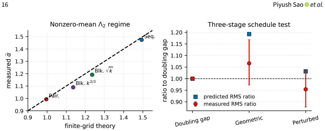
Optimal two-stage sequential blocking balances inner and outer accumulation: b ~ √k gives a k^{3/4} RMS exponent for centered inputs, and b ~ k^{2/3} gives a 7/6 exponent for noncentered inputs; fixed-stage hierarchies are geometric in the centered regime and follow a halving-gap schedule in the noncentered regime.
For independent centered inputs with unequal variances, the error-minimizing free assignment of leaves to tree positions is a variance-weighted prefix code, and the optimal cost lies between the entropy lower bound and the entropy-plus-one upper bound; measured penalties for pairwise and natural-order sequential trees are 1.79–3.37× and 55.5–106× the optimum, respectively.
In GEMM, the same kernel contraction ⟨K_T, G⟩ with G = (A^T A) ∘ (B B^T) controls the tree-dependent error; for centered random matrices, the RMS forward error relative to the absolute-value scale is Θ(u) for sequential FMA, Θ(uk^{-1/4}) for √k-blocked, and Θ(u√(log k/k)) for pairwise accumulation, with predictions matching measurements within 3% on the tested grid.
Because Λ1 and Λ2 require just one postorder traversal, any reduction routine can report its predicted typical error alongside its result; the paper demonstrates the workflow by extracting the actual tree of an array library's sum and predicting its measured RMS within 7% across sizes 27 to 2^20.

Reading between the lines

Editorial extensions of the paper, not claims the author makes directly.

Because the paper's dominance criterion uses only the ratio |μ|/τ and the tree statistics, a runtime could compute Λ1 and Λ2 during the reduction and automatically raise precision when the mean-to-deviation ratio crosses the threshold; the paper gives the criterion but stops short of implementing the policy.
The common-ancestor contraction should extend to other multi-way bilinear reductions — stencil computations, tensor contractions, batched inner products — whenever inputs carry a known second-moment matrix; testing it on correlated gradient reductions in low-precision training would be a direct next experiment.
The reported drift of the effective coefficient (0.217 down to 0.190) is consistent with the paper's own significand-based explanation, suggesting that a two-parameter model with a z^{-2} local-variance law might remove most of the configuration dependence that the constant-ν model leaves behind.
The measured cross-term covariances (5–10% of MSE) are small but not negligible; a correction term built from them could extend equation (1) to regimes where constant-ν currently breaks down, such as positive low-precision sums with stagnation and bias.

Share X Bluesky LinkedIn Reddit HN

Editorial analysis

A structured set of objections, weighed in public.

Desk editor's note, referee report, and a circularity audit.

Desk Editor's Note

read the letter

Worth a serious look. The paper gives a genuinely new handle on how reduction-tree geometry affects mean-square rounding error: the common-ancestor kernel K_T and its i.i.d. compression to Λ1 and Λ2. The exact recurrence under conditionally unbiased rounding is clean, and the optimization results — the k^{3/4} two-stage blocking, the geometric versus doubling-gap schedules, the Huffman import for variance-weighted depth — are well executed and clearly scoped. The GEMM extension via G=(A^T A)∘(BB^T) is a nice contraction, and the independent calibration work is about as careful as I have seen in this literature.

The soft spot is the constant-ν model itself. Under round-to-nearest it is an empirical approximation, not an exact consequence. The paper's own data show νeff drifting from 0.217 to 0.190, cross terms contributing 5–10% of MSE, and complete breakdown in low-precision positive sums due to stagnation and bias. The three-stage schedule ranking is not statistically confirmed: the paired bootstrap intervals contain unity. So the optimal-schedule theorems are model-relative; outside the calibrated regime they may not minimize actual MSE. That is a real limitation. But it is not a hidden one. The paper labels its claims 'under the constant-ν model', maps where the model fails, and the structural predictions — topology ordering, exponents, schedule rankings — are parameter-free functions of the tree statistics. The absolute level uses a calibrated ν, and the authors say so plainly.

One minor caveat: the stochastic-rounding diagnostics have a whiff of post-hoc selection (two initial misses, then follow-up runs), though the paper discloses this. It would be easy to overstate the confirmatory power there.

Who gets value from this? Numerical analysts and HPC practitioners who care about typical rounding error, schedule choice, or mixed-precision reductions. The paper deserves a serious referee, not a desk reject, and with reasonable revisions it would be a solid contribution.

Referee Report

0 major / 6 minor

Summary. This paper develops a second-moment theory for floating-point reduction trees. Under conditionally unbiased rounding with local variance νu²x² (the constant-ν model), the authors derive an exact recurrence for the accumulated error and show that the leading tree-dependent cost for a fixed input vector p is the quadratic form pᵀK_Tp, where K_T is the common-ancestor kernel counting shared internal ancestors. For i.i.d. inputs this cost reduces to τ²Λ₁(T)+μ²Λ₂(T), with Λ₁ total leaf depth and Λ₂ sum of squared internal subtree sizes. The paper then proves optimality results: balanced/sequential trees are the Λ₁ extrema; two-stage sequential blocking has RMS exponent 3/4 at block size √k; fixed-stage hierarchies have geometric schedules optimal for Λ₁ and a 'doubling-gap' schedule optimal for the polynomial order of Λ₂; and Huffman coding minimizes variance-weighted depth for heterogeneous centered inputs. The framework is extended to GEMM via a Hadamard-product contraction ⟨K_T,G⟩. Extensive experiments under round-to-nearest, using exact residuals and bitwise-validated tree extraction, support the topology ordering and absolute MSE levels within a few percent in tested regimes, while honestly documenting failure regimes (low-precision positive sums, stagnation, bias, and ν_eff drift).

Significance. The principal contribution is a clean, exact structural decomposition of the expected squared partial-sum cost in terms of the tree-only statistics Λ₁,Λ₂ and the input second-moment matrix. The kernel formulation is elegant and unifies summation, correlated inputs, and GEMM. The optimization results are model-relative but internally consistent, and the paper is unusually explicit about the empirical status of the constant-ν approximation. The experimental section is a model of reproducible numerical investigation: exact residual strategies per precision, bootstrap intervals, bitwise validation of the reconstructed NumPy tree, independent calibration of ν from node-local errors, and transparent reporting of inconclusive schedule comparisons and post-hoc stochastic-rounding checks. If the results hold, the paper provides a practical tool for predicting and comparing the typical error of reduction geometries.

minor comments (6)

[Section 2.4] The phrase 'the divisible case nb=k/b' is ambiguous: use n_b = k/b and define n_b as the number of blocks, with b the block size, so that the closed-form asymptotics in the following table are unambiguous.
[Appendix 1.1, Eq. (18)] The notation 'k^{3/4}=2c_p/c_a' is confusing because k already denotes the reduction size. Rename the crossover size (e.g., κ or k_*) and state that the crossover satisfies k_* = 2c_p/c_a.
[Section 3.1] The construction 'combine pairwise blocks of size g=k^{2-2α}' is degenerate at the endpoint α=1 (g=1). Please state separately that the sequential tree attains α=1.
[Table 2] In the row for stochastic rounding, 'stated grids 24–600' is vague. Please point to the exact grid definition (e.g., the Figure 9 caption) or list the sizes directly in the table.
[Section 3.4 / Section 6.5] The doubling-gap schedule is the Λ₂-optimal fixed-stage schedule under the constant-ν model; the direct experimental comparison (geometric vs. doubling-gap) is statistically inconclusive, with paired bootstrap intervals containing unity. The paper already discloses this in Section 6.5, but a one-sentence reminder at the end of Section 3.4 would help readers avoid over-reading the theorem as an empirical guarantee for round-to-nearest arithmetic.
[Figure 1] The kernel matrices displayed in the bottom panel are dense and hard to read in preprint form. Consider larger spacing, separate panel titles, or highlighting the diagonal and all-entry sums to improve legibility.

Circularity Check

0 steps flagged · score 0.0 of 10

No significant circularity: Eq. (1) is an algebraic consequence of the stated constant-ν model, ν is an explicitly calibrated coefficient validated out-of-sample, and all optimality results are parameter-free Λ1/Λ2 statistics.

full rationale

The derivation is not circular. The chain is: Theorem 2.2 derives an exact conditional second-moment recurrence from the definition of conditionally unbiased local errors; Corollary 2.3 specializes it by replacing ψ_v(x) with νu²x²; Proposition 2.4 rewrites Σ_v q_v² as pᵀK_Tp by an algebraic identity; Corollary 2.5 compresses the expectation to τ²Λ1(T)+μ²Λ2(T) for i.i.d. inputs. Eq. (1) is therefore a direct consequence of the model, not an input. The only fitted quantity is ν, and the paper is explicit that it is an empirical calibration parameter rather than an arithmetic constant: 'A fitted round-to-nearest value of ν serves as an empirical calibration parameter rather than an arithmetic constant' (Section 1, Layer 3). Calibration is out-of-sample: the summation ν=0.19 is pooled from a calibration grid and then applied to a different extracted NumPy tree ('With ν=0.19 fixed from the independent summation calibration, the model predicts the error within 7% across k=27,...,220'), and GEMM coefficients are 'calibrated from node-local errors independently of the root error used for validation' (Section 6.8). The summation calibration does use root MSE to define νeff (Section 6.7), but because the calibrated constant is then transferred across different tree topologies and sizes and checked against measured MSE and slopes, the prediction does not reduce to the fit by construction. The structural results (Propositions 3.1–3.4 and the Huffman Proposition 3.2) are parameter-free optimizations of Λ1/Λ2, proved from the tree statistics themselves or imported from external classical results (Huffman's theorem, Higham's blocked summation), not from author-specific prior claims; there are no load-bearing self-citations and no imported uniqueness theorems. The paper explicitly scopes its limitations—stagnation and bias in low precision (Section 6.2), νeff drift (Appendix 1.2), and model-relative optimality statements ('under the constant-ν model')—which are correctness/validity caveats, not circularity.

Assumptions & free parameters 3 free parameters · 6 assumptions · 1 invented entities

The central claim depends on the constant-ν model, a modeling assumption rather than a theorem; ν is empirically calibrated. Under stochastic rounding the recurrence is exact; under round-to-nearest the model is approximate with documented failure regimes.

free parameters (3)

ν (accumulation roundoff coefficient) = 0.19 (centered binary64); 0.15–0.25 range
Calibrated from node-local roundoff errors in Section 6.7; used for absolute-level predictions (Eq. 1) and noted to be configuration-dependent.
ν_a (GEMM accumulation coefficient) = 0.176–0.186
Independently calibrated from local accumulation errors for the GEMM grid (Section 6.8).
ν_p (GEMM product rounding coefficient) = 0.176–0.186
Independently calibrated for product rounding; contributes via the leaf term ν_p u_p² k in the GEMM model.

assumptions (6)

domain assumption Conditionally unbiased rounding with local variance ψ_v(x) (Definition 2.1)
Exact for stochastic rounding; used to derive Theorem 2.2; violated for deterministic round-to-nearest.
ad hoc to paper Constant-ν homogeneous variance model ψ_v(x) = νu²x² (Section 2.2)
Replaces operand-dependent variances by a single coefficient; the key approximation under round-to-nearest.
domain assumption Leading-order expansion h(T)u_a² ≪ 1 and ω^d ≈ 1 (Corollary 2.3)
Justifies dropping propagation weights; satisfied for binary64 but breaks in low precision.
ad hoc to paper Ensemble variance comparability (Assumption 1, Section 4.1)
Needed for the two-sided Θ claims in GEMM; excludes degenerate operands such as identity matrices.
domain assumption I.I.D. input second moment M = τ²I + μ²11ᵀ (Section 2.4)
Reduces the kernel contraction to the scalar statistics Λ₁ and Λ₂.
standard math Huffman optimality, entropy bounds, Schur product theorem, standard variance identities
Imported from information theory and matrix analysis for Propositions 3.2 and 4.3.

invented entities (1)

Common-ancestor kernel K_T independent evidence
purpose: Matrix-valued representation of reduction-tree cost satisfying pᵀK_Tp = Σ_v q_v²
A new mathematical object, directly computable from the tree and measurable through partial sums; validated in AR(1) tests (Section 6.4).

how reviews work

0 comments

Cite this review

Pith. "Pith review of A Second-Moment Theory for Floating-Point Reduction Trees." pith.science (2026). https://pith.science/paper/NSRMGBSN

@misc{pith2026260718758,
  author       = {Pith},
  title        = {Pith review of: A Second-Moment Theory for Floating-Point Reduction Trees},
  year         = {2026},
  howpublished = {\url{https://pith.science/paper/NSRMGBSN}},
  note         = {Machine review of arXiv:2607.18758}
}

read the original abstract

Summation error depends on partial-sum order, which standard worst-case bounds omit. To capture this dependence, we derive an exact mean-square error (MSE) recurrence for a binary reduction tree T under conditionally unbiased rounding. With unit roundoff u, the constant-nu model sets the local variance at pre-rounding value x to nu u^2 x^2. Its leading tree-dependent cost for the input vector p is p^T K_T p, where the common-ancestor kernel K_T counts the internal ancestors shared by each pair of leaves. For i.i.d. inputs of mean mu and variance tau^2, this expected cost is tau^2 Lambda_1(T) + mu^2 Lambda_2(T), where Lambda_1 is total leaf depth and Lambda_2 sums squared internal-subtree sizes; Lambda_1 governs centered inputs, while Lambda_2 captures nonzero means. We use these statistics to characterize optimal tree topologies and schedules. Balanced and sequential trees attain the centered extrema. For k inputs, optimal two-stage sequential blocking yields root-mean-square (RMS) error scaling as k^{3/4}. For fixed-stage hierarchies, geometric schedules are optimal for centered inputs, whereas the optimal noncentered stage exponents halve successively. For independent centered inputs with unequal variances, Huffman coding minimizes variance-weighted depth over free leaf assignments. We extend the kernel to matrix multiplication through operand Gram matrices. We then test the approximation under round-to-nearest using exact residuals. Across binary64, binary32, and software-emulated binary16 and bfloat16, the model recovers the ordering among tree topologies; K_T tracks AR(1) partial-sum costs. For GEMM, independently calibrated predictions differ from measurements by at most 3% on the tested grid. A reduction tree extracted from an array library predicts the measured RMS scaling. However, stagnation and bias in positive low-precision sums limit the model's applicability.

Figures

Figures reproduced from arXiv: 2607.18758 by the authors.

**Figure 1.** Shared ancestry determines the second-moment cost for three reduction trees on the same k = 8 inputs. Top: each internal-node label is its subtree size |L (v)|; the blocked tree accumulates sequentially within blocks and across block totals. Bottom: (KT)ij counts the internal ancestors shared by leaves i and j. The displayed diagonal and all-entry sums give Λ1 = tr KT and Λ2 = 1 ⊤KT1. Thus the sequential and blocked… view at source ↗

**Figure 2.** Dominance boundary for i.i.d. pure summation. Each curve connects exact values of |µ|/τ = √︁ Λ1/Λ2: integer sizes for sequential trees, powers of two for pairwise trees, and square sizes k = b 2 for two-stage blocked trees. Above a curve, the µ 2Λ2 term exceeds τ 2Λ1 for that family; below it, the reverse holds. The marked k = 4096 thresholds are 0.019 (sequential) and 0.038 (pairwise). The workload labels illustrat… view at source ↗

**Figure 3.** Tree family and stage schedule jointly determine the RMS power law. Left: exact √ Λ1 for sequential, fixed-b = 32 blocked, optimized two-stage blocked, three-stage geometric, and pairwise families. The fixed-b curve has local slope 3/4 at k = b 2 and approaches slope one, whereas b ≍ √ k retains exponent 3/4. Right: centered exponents ατ from Λ1 and noncentered exponents αµ from Λ2; the two- and three-stage noncente… view at source ↗

Figures from the paper (11 more)

**Figure 4.** Figure 4: Left: fitted centered-normal slopes with bootstrap 95% intervals over k = 64, . . . , 8192; black ticks are finite-grid fits of √ Λ1. Right: fitted slopes for uniform [0, 1] inputs in software binary16 and bfloat16; black ticks are the noncentered finite-grid slopes of…

**Figure 5.** Figure 5: Binary64 round-to-nearest, centered inputs. Left: four overlapping fit windows for fixed b = 32. Right: block growth b ≍ k β. Error bars are bootstrap 95% intervals; dashed curves are finite-grid or asymptotic tree-statistic predictions. Section 6.3 discusses the fixed…

**Figure 6.** Figure 6: First-order autoregressive (AR(1)) inputs. The full common-ancestor kernel tracks the empirical partial-sum cost (left), while the i.i.d. Λ1 compression departs from the empirical cost as correlation increases (right, logarithmic scale). Section 6.4 discusses the corre…

**Figure 7.** Figure 7: Variance-weighted leaf-depth costs for two heterogeneous profiles (k = 256). The shaded interval is the entropy bracket [WH2 (w),W{H2 (w) + 1}]; labels above the bars give exact-reference round-to-nearest MSE coefficients. Proposition 3.2 gives the bracket, and Section…

**Figure 8.** Figure 8: Left: noncentered normal fitted slopes versus exact finite-grid tree-statistic slopes. Right: deterministic and measured three-stage schedule ratios. The predicted RMS ratio is √︃ Λ2/Λ2,dg; measured error bars are paired bootstrap 95% intervals. Section 6.5 discusses t…

**Figure 9.** Figure 9: Measured stochastic-rounding second moment divided by the exact nodewise recurrence. Circles show all six initial bootstrap 95% intervals; open squares show post-hoc larger-sample diagnostics for the two initial misses. Section 6.6 discusses the initial and diagnostic…

**Figure 10.** Figure 10: Left: effective centered binary64 MSE coefficient across size, tree, and input distribution, with three reference levels. Right: normalized local second moment versus significand; a horizontal value of one is the uniform-in-cell prediction. Section 6.7 discusses the c…

**Figure 11.** Figure 11: Fused multiply–add (FMA) and separate product/addition rounding. Left: measured MSE divided by the independently calibrated two-term model. Right: RF, the ratio of RMS quantities. Error bars are bootstrap 95% intervals. Section 6.8 discusses the independent calibratio…

**Figure 13.** Figure 13: Local non-FMA dot-product slopes and the curve from independently calibrated product and accumulation coefficients. The derivation appears in Appendix 1.1. [2] Eric Hallman and Ilse C. F. Ipsen. “Precision-aware deterministic and probabilistic error bounds for floati…

**Figure 12.** Figure 12: Measured exact-reference RMS error of contiguous binary64 np.sum, the prediction from the extracted tree using the independently calibrated ν = 0.19, and the idealized pure-pairwise prediction. Section 5.1 sketches the extracted hierarchy. Shading is the bootstrap 9…

**Figure 14.** Figure 14: Four-stage round-to-nearest scaling experiment. Left: measured RMS and the √ Λ1 curve scaled at the first point; their finitegrid slopes are 0.602 and 0.619. Right: νeff = MSE/(u 2Λ1) with bootstrap 95% intervals. Its decrease from 0.217 to 0.190 across the grid acco…

Discussion (0). Sign in to comment.

Reference graph

Works this paper leans on

37 extracted references · 9 canonical work pages

[1]

A New Approach to Probabilistic Rounding Error Analysis

Nicholas J. Higham and Theo Mary. “A New Approach to Probabilistic Rounding Error Analysis”. In:SIAM Journal on Scientific Computing41.5 (2019), A2815–A2835.DOI: 10.1137/ 18M1226312. 102 103 104 105 106 k 10−15 10−14 10−13 RMS error Predicting np.sum from its tree measured extracted tree pure pairwise Figure 12.Measured exact-reference RMS error of contig...

2019
[2]

Precision-aware determin- istic and probabilistic error bounds for floating point summa- tion

Eric Hallman and Ilse C. F. Ipsen. “Precision-aware determin- istic and probabilistic error bounds for floating point summa- tion”. In:Numerische Mathematik155.1–2 (2023), pp. 83–119. DOI: 10.1007/s00211-023-01370-y

doi:10.1007/s00211-023-01370-y 2023
[3]

The Ancestral Matrix of a Rooted Tree

Eric O. D. Andriantiana, Kenneth Dadedzi, and Stephan Wag- ner. “The Ancestral Matrix of a Rooted Tree”. In:Linear Algebra and its Applications575 (2019), pp. 35–65.DOI: 10.1016/j.laa. 2019.04.004

doi:10.1016/j.laa 2019
[4]

A Method for the Construction of Minimum-Redundancy Codes

David A. Huffman. “A Method for the Construction of Minimum-Redundancy Codes”. In:Proceedings of the IRE40.9 (1952), pp. 1098–1101.DOI: 10.1109/JRPROC.1952.273898

arXiv 1952
[5]

Cover and Joy A

Thomas M. Cover and Joy A. Thomas.Elements of Information Theory. 2nd ed. Wiley-Interscience, 2006.ISBN: 978-0-471- 24195-9.DOI: 10.1002/047174882X

doi:10.1002/047174882x 2006
[6]

Linear-Time Approximation Algorithms for Computing Numerical Summation with Prov- ably Small Errors

Ming-Yang Kao and Jie Wang. “Linear-Time Approximation Algorithms for Computing Numerical Summation with Prov- ably Small Errors”. In:SIAM Journal on Computing29.5 (2000), pp. 1568–1576.DOI: 10.1137/S0097539798341594

work page doi:10.1137/s0097539798341594 2000
[7]

A Fast Al- gorithm for Optimal Length-Limited Huffman Codes

Lawrence L. Larmore and Daniel S. Hirschberg. “A Fast Al- gorithm for Optimal Length-Limited Huffman Codes”. In: Journal of the ACM37.3 (1990), pp. 464–473.DOI: 10.1145/ 79147.79150

arXiv 1990
[8]

The Accuracy of Floating Point Sum- mation

Nicholas J. Higham. “The Accuracy of Floating Point Sum- mation”. In:SIAM Journal on Scientific Computing14.4 (1993), pp. 783–799.DOI: 10.1137/0914050

doi:10.1137/0914050 1993

Show all 37 references

[9]

A Class of Fast and Accurate Summation Algorithms

Pierre Blanchard, Nicholas J. Higham, and Theo Mary. “A Class of Fast and Accurate Summation Algorithms”. In:SIAM Journal on Scientific Computing42.3 (2020), A1541–A1557.DOI: 10.1137/19M1257780

2020 doi
[10]

Reducing Floating Point Error in Dot Prod- uct Using the Superblock Family of Algorithms

Anthony M. Castaldo, R. Clint Whaley, and Anthony T. Chronopoulos. “Reducing Floating Point Error in Dot Prod- uct Using the Superblock Family of Algorithms”. In:SIAM Journal on Scientific Computing31.2 (2009), pp. 1156–1174.DOI: 10.1137/070679946. Floating-Point Reduction Tre...

2009 doi
[11]

Revealing Floating-Point Accumulation Orders in Software/Hardware Implementations

Peichen Xie et al. “Revealing Floating-Point Accumulation Orders in Software/Hardware Implementations”. In:2025 USENIX Annual Technical Conference (USENIX ATC 25). Boston, MA: USENIX Association, July 2025, pp. 1425–1440. ISBN: 978-1-939133-48-9.URL: https : / / www . usenix ....

2025
[12]

Ver- sion 1.26.4

NumPy contributors.NumPy 1.26.4 source: pairwise_sum in numpy/core/src/umath/loops_utils.h.src. Ver- sion 1.26.4. The 8192-element chunking arises from the ufunc reduction buffer, whose size is controlled by numpy.setbufsize, outside the pairwise-summation routine. NumPy. Feb....

2024
[13]

Mixed Precision Training

Paulius Micikevicius et al. “Mixed Precision Training”. In:6th International Conference on Learning Representations (ICLR 2018)

2018
[14]

NumPy pull request 31274; merged 29 April 2026; released in NumPy 2.5.0 on 21 June 2026

Pieter Eendebak.ENH: fast path for full contiguous reductions. NumPy pull request 31274; merged 29 April 2026; released in NumPy 2.5.0 on 21 June 2026. NumPy. Apr. 19, 2026.URL: https://github.com/numpy/numpy/pull/31274 (visited on 07/20/2026)

2026
[15]

Higham.Accuracy and Stability of Numerical Algo- rithms

Nicholas J. Higham.Accuracy and Stability of Numerical Algo- rithms. 2nd ed. SIAM, 2002.DOI: 10.1137/1.9780898718027

2002 doi
[16]

Algorithms for arbitrary precision floating point arithmetic

Douglas M. Priest. “Algorithms for arbitrary precision floating point arithmetic”. In:Proceedings of the 10th IEEE Symposium on Computer Arithmetic. IEEE Computer Society Press, 1991, pp. 132–143.DOI: 10.1109/ARITH.1991.145549

1991
[17]

Fast and Accurate Floating Point Summation with Application to Computational Geome- try

James Demmel and Y ozo Hida. “Fast and Accurate Floating Point Summation with Application to Computational Geome- try”. In:Numerical Algorithms37.1–4 (2004), pp. 101–112.DOI: 10.1023/B:NUMA.0000049458.99541.38

2004
[18]

Accu- rate Sum and Dot Product

Takeshi Ogita, Siegfried M. Rump, and Shin’ichi Oishi. “ Accu- rate Sum and Dot Product”. In:SIAM Journal on Scientific Com- puting26.6 (2005), pp. 1955–1988.DOI: 10.1137/030601818

2005 doi
[19]

Numerical reproducibility for the parallel reduction on multi- and many-core architectures

Caroline Collange et al. “Numerical reproducibility for the parallel reduction on multi- and many-core architectures”. In: Parallel Computing49 (2015), pp. 83–97.DOI: 10.1016/j.parco. 2015.09.001

2015 doi
[20]

Best “Or- dering

Thomas G. Robertazzi and Stephen C. Schwartz. “Best “Or- dering” for Floating-Point Addition”. In:ACM Transactions on Mathematical Software14.1 (1988), pp. 101–110.DOI: 10.1145/ 42288.42343

1988
[21]

On Floating-Point Summation

Terje O. Espelid. “On Floating-Point Summation”. In:SIAM Review37.4 (1995), pp. 603–607.DOI: 10.1137/1037130

1995 doi
[22]

Numerical inverting of matrices of high order

John von Neumann and Herman H. Goldstine. “Numerical inverting of matrices of high order”. In:Bulletin of the American Mathematical Society53.11 (1947), pp. 1021–1099.DOI: 10.1090/ S0002-9904-1947-08909-6

1947
[23]

Test of probabilistic models for the propagation of roundoff errors

Peter Henrici. “Test of probabilistic models for the propagation of roundoff errors”. In:Communications of the ACM9.6 (1966), pp. 409–410.DOI: 10.1145/365696.365698

1966
[24]

Tests of probabilistic models for propagation of roundoff errors

T. E. Hull and J. R. Swenson. “Tests of probabilistic models for propagation of roundoff errors”. In:Communications of the ACM9.2 (1966), pp. 108–113.DOI: 10.1145/365170.365212

1966
[25]

On roundoff error distributions in floating point and logarithmic arithmetic

Jesse L. Barlow and Erwin H. Bareiss. “On roundoff error distributions in floating point and logarithmic arithmetic”. In: Computing34.4 (1985), pp. 325–347.DOI: 10.1007/BF02251833

1985 doi
[26]

A proba- bilistic round-off error propagation model. Application to the eigenvalue problem

Françoise Chatelin and Marie-Christine Brunet. “A proba- bilistic round-off error propagation model. Application to the eigenvalue problem”. In:Reliable Numerical Computation. Ed. by M. G. Cox and S. Hammarling. Oxford University Press, 1990, pp. 139–160.DOI: 10.1093/oso/97801...

1990
[27]

Stochastic Rounding and Its Probabilistic Backward Error Analysis

Michael P. Connolly, Nicholas J. Higham, and Theo Mary. “Stochastic Rounding and Its Probabilistic Backward Error Analysis”. In:SIAM Journal on Scientific Computing43.1 (2021), A566–A585.DOI: 10.1137/20M1334796

2021 doi
[28]

Stochastic rounding: implementation, error analysis and applications

Matteo Croci et al. “Stochastic rounding: implementation, error analysis and applications”. In:Royal Society Open Science9.3 (2022), p. 211631.DOI: 10.1098/rsos.211631

2022 doi
[29]

Stochastic Rounding Variance and Probabilistic Bounds: A New Approach

El-Mehdi El Arar et al. “Stochastic Rounding Variance and Probabilistic Bounds: A New Approach”. In:SIAM Journal on Scientific Computing45.5 (2023), pp. C255–C275.DOI: 10.1137/ 22M1510819

2023
[30]

Minimizing Roundoff Errors of Prefix Sums via Dynamic Construction of Huffman Trees

Ming-Yang Kao and Jie Wang. “Minimizing Roundoff Errors of Prefix Sums via Dynamic Construction of Huffman Trees”. In:Theoretical Computer Science262.1–2 (2001), pp. 101–115. DOI: 10.1016/S0304-3975(00)00183-3

2001 doi
[31]

Fast Reproducible Floating-Point Summation

James Demmel and Hong Diep Nguyen. “Fast Reproducible Floating-Point Summation”. In:2013 IEEE 21st Symposium on Computer Arithmetic. IEEE, 2013, pp. 163–172.DOI: 10.1109/ ARITH.2013.9. 20 Piyush Sao et al

2013
[32]

Reproducible and Accurate Matrix Multiplication

Roman Iakymchuk et al. “Reproducible and Accurate Matrix Multiplication”. In:Scientific Computing, Computer Arithmetic, and V alidated Numerics. V ol. 9553. Lecture Notes in Com- puter Science. Cham: Springer International Publishing, 2016, pp. 126–137.DOI: 10.1007/978-3-319-3...

2016 doi
[33]

A Statistical Analysis of Error in MPI Reduction Operations

Samuel D. Pollard and Boyana Norris. “A Statistical Analysis of Error in MPI Reduction Operations”. In:2020 IEEE/ACM 4th International W orkshop on Software Correctness for HPC Applications (Correctness). 2020, pp. 49–57.DOI: 10 . 1109 / CORRECTNESS51934.2020.00011

2020
[34]

Mixed Precision Block Fused Multiply- Add: Error Analysis and Application to GPU Tensor Cores

Pierre Blanchard et al. “Mixed Precision Block Fused Multiply- Add: Error Analysis and Application to GPU Tensor Cores”. In:SIAM Journal on Scientific Computing42.3 (2020), pp. C124– C141.DOI: 10.1137/19M1289546

2020 doi
[35]

Deep Learning with Limited Numerical Precision

Suyog Gupta et al. “Deep Learning with Limited Numerical Precision”. In:Proceedings of the 32nd International Conference on Machine Learning. V ol. 37. Proceedings of Machine Learning Research. 2015, pp. 1737–1746.URL: https://proceedings.mlr. press/v37/gupta15.html

2015
[36]

El-Mehdi El Arar et al.Probabilistic Error Analysis of Limited- Precision Stochastic Rounding: Horner’s Algorithm and Pairwise Summation. Mar. 25, 2026.DOI: 10.48550/arXiv.2603.24161. arXiv: 2603.24161 [math.NA].URL: https://arxiv.org/abs/2603. 24161 (visited on 07/20/2026)

2026 doi
[2018]

net/forum?id=r1gs9JgRZ

arXiv: 1710.03740 [cs.AI].URL: https://openreview. net/forum?id=r1gs9JgRZ

arXiv

Pith tools

Reviewed August 1, 2026 · model on record in the stance chip above.

[1] [1]

A New Approach to Probabilistic Rounding Error Analysis

Nicholas J. Higham and Theo Mary. “A New Approach to Probabilistic Rounding Error Analysis”. In:SIAM Journal on Scientific Computing41.5 (2019), A2815–A2835.DOI: 10.1137/ 18M1226312. 102 103 104 105 106 k 10−15 10−14 10−13 RMS error Predicting np.sum from its tree measured extracted tree pure pairwise Figure 12.Measured exact-reference RMS error of contig...

2019

[2] [2]

Precision-aware determin- istic and probabilistic error bounds for floating point summa- tion

Eric Hallman and Ilse C. F. Ipsen. “Precision-aware determin- istic and probabilistic error bounds for floating point summa- tion”. In:Numerische Mathematik155.1–2 (2023), pp. 83–119. DOI: 10.1007/s00211-023-01370-y

doi:10.1007/s00211-023-01370-y 2023

[3] [3]

The Ancestral Matrix of a Rooted Tree

Eric O. D. Andriantiana, Kenneth Dadedzi, and Stephan Wag- ner. “The Ancestral Matrix of a Rooted Tree”. In:Linear Algebra and its Applications575 (2019), pp. 35–65.DOI: 10.1016/j.laa. 2019.04.004

doi:10.1016/j.laa 2019

[4] [4]

A Method for the Construction of Minimum-Redundancy Codes

David A. Huffman. “A Method for the Construction of Minimum-Redundancy Codes”. In:Proceedings of the IRE40.9 (1952), pp. 1098–1101.DOI: 10.1109/JRPROC.1952.273898

arXiv 1952

[5] [5]

Cover and Joy A

Thomas M. Cover and Joy A. Thomas.Elements of Information Theory. 2nd ed. Wiley-Interscience, 2006.ISBN: 978-0-471- 24195-9.DOI: 10.1002/047174882X

doi:10.1002/047174882x 2006

[6] [6]

Linear-Time Approximation Algorithms for Computing Numerical Summation with Prov- ably Small Errors

Ming-Yang Kao and Jie Wang. “Linear-Time Approximation Algorithms for Computing Numerical Summation with Prov- ably Small Errors”. In:SIAM Journal on Computing29.5 (2000), pp. 1568–1576.DOI: 10.1137/S0097539798341594

work page doi:10.1137/s0097539798341594 2000

[7] [7]

A Fast Al- gorithm for Optimal Length-Limited Huffman Codes

Lawrence L. Larmore and Daniel S. Hirschberg. “A Fast Al- gorithm for Optimal Length-Limited Huffman Codes”. In: Journal of the ACM37.3 (1990), pp. 464–473.DOI: 10.1145/ 79147.79150

arXiv 1990

[8] [8]

The Accuracy of Floating Point Sum- mation

Nicholas J. Higham. “The Accuracy of Floating Point Sum- mation”. In:SIAM Journal on Scientific Computing14.4 (1993), pp. 783–799.DOI: 10.1137/0914050

doi:10.1137/0914050 1993