REVIEW 4 major objections 5 minor 27 references
Extremal eigenvalues of sample covariance matrices with general population
T0 review · 4 major / 5 minor · reviewed 2026-08-14 · deepseek-v4-flash
Pith's one-line read Above a critical sample-to-population ratio, the largest eigenvalues of a sample covariance matrix are governed by the population's own order statistics and converge to a Weibull law.
desk verdict Settles the Weibull/Gaussian edge transition for sample covariance matrices with convex population decay; the main i.i.d. result is solid, while the deterministic-Σ scope is conditional on an intricate assumed event. read the letter →
The pith
A machine-rendered reading of the paper's core claim, the machinery that carries it, and where it could break.
The reading
What carries the argument
The argument runs through the deformed Marchenko-Pastur equation for the Stieltjes transform, m_fc(z) = { -z + $d^{{-1}}$ int t dnu(t)/(1+t m_fc(z)) }^{-1}. The threshold d_+ is read off when the quantity H(tau)=$d^{{-1}}$ int $t^{2}$ dnu(t)/((Re tau + t)^2 + (Im tau)^2) at tau=-1 equals d_+/d<1, marking the absence of spectrum outside the bulk and pinning the right edge at L_+=1+tau_+. Near the edge, 1/m_fc(z) is approximately linear in z, 1/m_fc(z)=-1 + d/(d-d_+)(L_+-z) + O((log M)(kappa+eta)^{min{b,2}}), which converts the location of sample eigenvalues into the population order statistics. The technical core is a local law comparing the resolvent's normalized trace m(z) to a random object \hat{m}_fc(z) defined from the empirical population spectrum, using a block linearization H(z)=[[-z I_N, X^*],[X, -$Sigma^{{-1}}$]] and fluctuation averaging to control the imaginary part of m down to scales below $N^{{-1/2}}$; because the limiting density has no square-root edge, the usual stability bound is replaced by the good-configuration assumptions on Sigma.
What would settle it
Run the numerical experiment at increasing M with a fixed population density (1-t)^b on [l,1], b>1, and d>d_+; collect the top eigenvalue lambda_1 over many trials and compare the empirical distribution of $M^{{1/(b+1)}}$(L_+-lambda_1) with G_{b+1}(s) using the stated C_nu. The claim fails if the fit does not stabilize to that Weibull shape and scale, or if the joint distribution of the top gamma gaps does not match the order-statistics distribution with scaling C_d; a second check is that for d just below d_+ the fluctuations remain of order $M^{{-1/2}}$ and Gaussian.
Extended reading notes
Core claim
The central claim is Theorem 2.8: under a good-configuration assumption on the top eigenvalues of Sigma, for d>d_+ the joint distribution of $M^{{1/(b+1)}}$(L_+-lambda_i) for i=1,...,gamma converges to the joint distribution of C_d $M^{{1/(b+1)}}$(1-sigma_i), where C_d=(d-d_+)/d. In particular, for i.i.d. population entries the largest eigenvalue of Q satisfies the Weibull limit G_{b+1}(s)=1-exp(-C_nu $s^{{b+1}}$/(b+1)) with C_nu=(d/(d-d_+))^{b+1} lim_{t->1} rho_nu(t)/(1-t)^b. Theorem 2.7 locates the right edge at L_+=1+tau_+ and shows that the limiting density of Q decays like kappa^b at distance kappa from the edge, and Theorem 2.9 gives a centered Gaussian limit of size $M^{{-1/2}}$ for d<d_+ when the population eigenvalues are i.i.d., with variance ($d^{2}$ M)^{-1}(int |t tau/(t+tau)|^2 dnu(t) - (int t tau/(t+tau) dnu(t))^2).
Load-bearing premise
The whole comparison rests on the good-configuration event $\Omega$: the largest n0 eigenvalues of Sigma must be separated from each other and from the edge 1 by gaps of order $M^{{-1/(b+1)}}$ but not much larger, and the averaged sums involving Sigma must converge to the limiting integrals; if those gaps are missing, the sample eigenvalues are not matched one-to-one to population order statistics and the Weibull conclusion can fail.
Editorial extensions
If this is right
- For d>d_+, the top gamma sample eigenvalues are asymptotically the same random object as the top gamma population eigenvalues, rescaled by C_d; the largest eigenvalue is Weibull with exponent b+1 rather than Tracy-Widom.
- The sample spectral density has convex decay at the right edge, mu_fc(L_+-kappa) ~ kappa^b, so the local edge regime changes its behavior when the ratio d crosses d_+.
- The boundary d_+ = int t^2 (1-t)^{-2} dnu(t) is explicit in the population law, so one can predict from Sigma alone which regime a dataset is in.
- Under Gaussian sampling the same results hold for non-diagonal Sigma, so the finding is not an artifact of the diagonal model.
- Corollary 4.10 gives quantitative rates, with errors involving M^{3phi}/M^b and (log M)^2/M^{1/(b+1)} plus the bad-configuration probability (log M)^{1+2b}/M^phi.
Reading between the lines
- The paper does not discuss what happens when the top population gaps are far smaller than M^{-1/(b+1)}; a natural expectation is that the one-to-one order-statistics matching breaks and a spiked or BBP-type regime takes over, since the good-configuration event explicitly excludes that case.
- The exponent b+1 in the Weibull law makes the effective tail index of the population edge; for fixed d>d_+, a smaller b gives heavier tails in the rescaled largest eigenvalue, which is a testable prediction for simulations.
- The same peak-tracking mechanism via the imaginary part of the resolvent may transfer to other ensembles whose limiting density has non-square-root edge decay, beyond the deformed Wigner and sample covariance settings treated here.
- The sharp scale change from M^{-1/2} Gaussian fluctuations below d_+ to M^{-1/(b+1)} Weibull fluctuations above d_+ suggests a genuine phase transition in the fluctuation size; checking the transition width near d_+ numerically would be a natural follow-up.
Signed reviews
Editorial analysis
A structured set of objections, weighed in public.
Referee Report
Summary. The paper studies the extremal eigenvalues of sample covariance matrices Q = (Σ^{1/2}X)(Σ^{1/2}X)^* for M×N random X with independent entries and a diagonal population covariance Σ. Under the assumption that the limiting spectral density of Σ has the Jacobi form ρ_ν(t) ∝ (1−t)^b f(t) with b>1, the authors define a threshold d_+ = ∫ t^2 (1−t)^{-2} dν(t). For d>d_+, they claim that the right edge of the LSD of Q has convex decay and that the γ largest eigenvalues of Q, rescaled by M^{1/(b+1)}, converge to the corresponding order statistics of Σ, with an explicit Weibull limit for the largest eigenvalue. For d<d_+, they claim a Gaussian fluctuation at scale M^{-1/2} when the entries of Σ are i.i.d. The proof uses the deformed Marchenko–Pastur equation, a local law near the edge, fluctuation averaging, and an intermediate random object \mhat m_fc that depends on Σ. The main theorems are stated under a 'good configuration' event Ω that encodes spacing of the top population eigenvalues, a non-resonance condition, and an averaged convergence condition.
Significance. If the results are correct, the paper provides a sharp phase transition for the edge behavior of sample covariance matrices with general population: above d_+ the largest eigenvalues follow the population order statistics with a Weibull limit, and below d_+ the fluctuation is Gaussian. The constants d_+, C_d, and C_ν are explicit functionals of the population law ν, and no parameter is fitted. The paper also extends the deformed-Wigner extremal-eigenvalue strategy to the sample covariance setting, which is a technically substantial step. However, the manuscript currently leaves several load-bearing estimates and verifications to analogies or external references, so the significance can be fully assessed only after these gaps are filled.
major comments (4)
- [§4.1, Theorem 2.7] The proof of the density bound (2.19) is omitted: the text says the proof is analogous to Lemma A.4 of [18] and gives no details. This bound is load-bearing because it is used in Appendix A, Lemma A.5, to control Im m_fc, which in turn supports the verification of condition (2.14) and the estimates in §5. Without a full proof of (2.19), the convex-decay assertion that is the basis for the order-statistic and Weibull results is not established within the manuscript.
- [§4.4 and Assumption 2.6(i), condition (2.16)] The deterministic-Σ case is advertised in the abstract as holding 'with some additional assumptions,' but the only such assumption is the un-verified event Ω of Definition 2.5, in particular the uniform averaged convergence condition (2.16). This condition is exactly what bounds the first term in (4.32), and it is also needed for Lemma 4.4 and Proposition 5.1. For i.i.d. Σ, Lemma A.3 verifies a stronger form, but for deterministic Σ satisfying only ESD convergence and spacing conditions, (2.16) is an additional non-explicit hypothesis. The theorem is therefore conditional on a hypothesis that is not derived from any more primitive deterministic condition, and the deterministic scope claimed in the abstract is not actually established.
- [§4.5, proof of Theorem 2.9] The crucial estimate |L_+ − λ_1| ≺ M^{-2/3} is obtained by asserting that the model satisfies Condition 1.1 of [3] and then applying Theorem 4.1 of [3]. No verification of Condition 1.1 is given, and the text only says that 'adapting the idea of the proof of Lemma A.4 in [18]' yields the needed bounds. This step is essential: without |L_+ − λ_1| ≺ M^{-2/3}, the Gaussian fluctuation of λ_1 cannot be identified with that of \hat L_+, which is the point of Theorem 2.9. A complete proof must either verify Condition 1.1 of [3] explicitly or provide a self-contained derivation of the M^{-2/3} bound.
- [Lemma 4.1(4.12), Corollary 5.11, Lemma 6.11, and Appendix A] Several proofs that are used directly in the main argument are deferred or omitted. The second part of Lemma 4.1 is stated to be 'analogous'; Corollary 5.11 is said to follow as in [19] without proof; Lemma 6.11, the fluctuation averaging lemma, is proved only by saying that the method of [19] or [10] applies; and Lemma A.3 in Appendix A refers to Theorem 8.2 of [19] for 'the left parts.' Since these estimates are load-bearing for the local law and eigenvalue tracking, the manuscript currently does not allow the reader to verify the central claims without consulting the cited works in detail.
minor comments (5)
- [Abstract and Section 1] The abstract contains the undefined symbol '\caQ' in 'the largest eigenvalue of \caQ'; this should be Q. Also, the sentence 'in the limit M, N → ∞ with N/M → d ∈ (0,∞)' later assumes \hat d is constant; the distinction between \hat d and d should be clarified.
- [§2.2, Definition 2.5] In condition (2.10), the spacing bound uses '(log M)κ_0' but the later estimate (2.17) in the i.i.d. case and Corollary 4.10 contain powers of log M; it would help to state explicitly whether the constants in Definition 2.5 are allowed to vary with n_0, since n_0 is fixed.
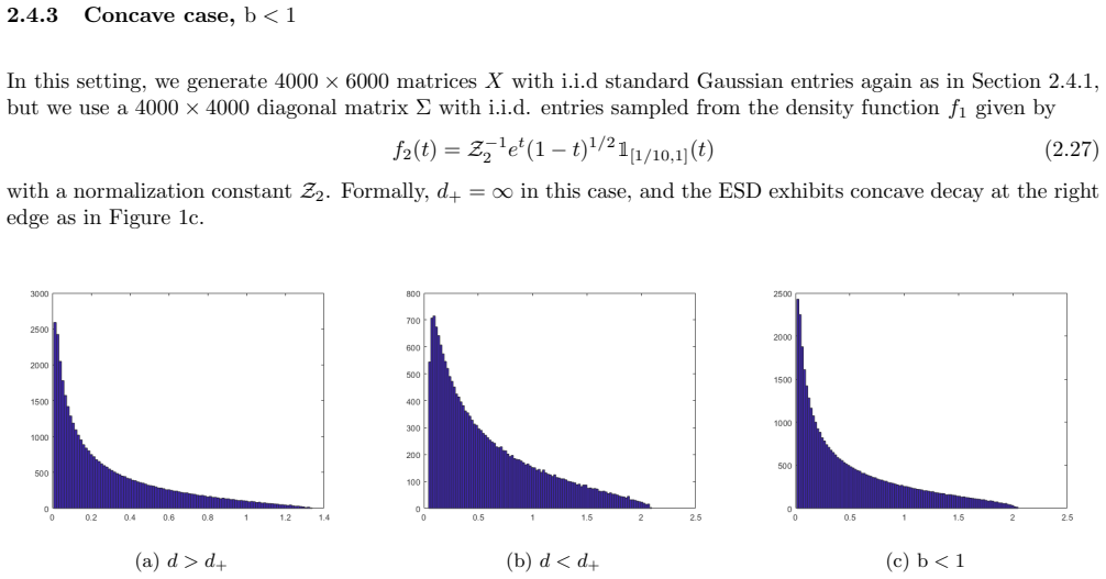
- [§2.4, numerical experiments] The text refers to Figure 1 for the histograms, but the figure is not reproduced in the manuscript text; the reader cannot assess the numerical evidence. If this is an artifact of the submission format, the figure legend should at least describe the axes and the observed decay qualitatively.
- [§5.3, Lemma 5.10] The word 'follwing' appears in the sentence before Lemma 5.9; this is a typo. Also, in Corollary 5.11, the bound (5.91) is stated for 'γ ∈ J1,n0−1K' but the sum is over α ∈ Jn0,MK with α≠γ; the latter range already excludes γ, so the condition α≠γ is redundant but harmless.
- [Appendix A, Lemma A.1 and Lemma A.3] The statements say 'sample points distributed according to ν' but do not explicitly say 'i.i.d.'; since the appendix is used only for the i.i.d. case, making this explicit would prevent confusion with the deterministic case in Assumption 2.6.
Circularity Check
No significant circularity: all constants are explicit functionals of the population law ν; the only caveat is an explicit good-configuration assumption for deterministic Σ.
full rationale
The derivation chain is self-contained against the stated hypotheses. The supercritical edge location L+ and threshold d+ are explicit functionals of ν (Theorem 2.7, Eq. (2.18)), and the Weibull constant Cν in (2.23) is an explicit functional of ν; nothing is fitted. The proof of Theorem 2.8 proceeds by comparing the resolvent of Q to the deterministic m_fc via an intermediate random object ȷm_fc; the eigenvalue location estimate (4.49) follows from Lemma 4.1 (a first-order expansion of 1/m_fc near the edge), Lemma 4.4 (the bound on |1/ȷm_fc - 1/m_fc|), and Proposition 4.7 (locating the eigenvalue via the peak of Im m). None of these steps assumes the target joint distribution; the target enters only through the population order statistics, whose Weibull limit is supplied by Fisher–Tippett–Gnedenko. The good-configuration event Ω in Definition 2.5 is a collection of explicit gap and fluctuation hypotheses; for i.i.d. Σ it is verified in Appendix A, while for deterministic Σ it is stated as Assumption 2.6(i). This is a transparent additional hypothesis, not a circularity. Citations to [18] and [19] supply technical tools (stability analysis of self-consistent equations, fluctuation averaging, order-statistic gap bounds); they are external published results with parameter-free hypotheses and do not re-import the conclusion of this paper. The deterministic-Σ caveat raised by the skeptic is a limitation in advertised scope, not a circular reduction: condition (2.16) is assumed, not derived from the theorem being proved. Overall circularity score 0.
Assumptions & free parameters
assumptions (4)
- standard math The deformed Marchenko-Pastur equation (3.5) has a unique solution in the upper half-plane, which is the Stieltjes transform of the LSD of Q.
- domain assumption The population spectral measure ν has density Z^{-1}(1-t)^b f(t) on [l,1] with b>1 and f in C^1 positive on [l,1].
- domain assumption The entries of X are independent, centered, have variance 1/N and satisfy the moment bound E|x_ij|^p ≤ c_p N^{-p/2}.
- ad hoc to paper For deterministic or non-i.i.d. random Σ, the event Ω of Definition 2.5 holds; for i.i.d. Σ with law ν it holds with probability tending to 1.
Cite this review
Pith. "Pith review of Extremal eigenvalues of sample covariance matrices with general population." pith.science (2026). https://pith.science/paper/NTIC7CIL
@misc{pith2026190807444,
  author       = {Pith},
  title        = {Pith review of: Extremal eigenvalues of sample covariance matrices with general population},
  year         = {2026},
  howpublished = {\url{https://pith.science/paper/NTIC7CIL}},
  note         = {Machine review of arXiv:1908.07444}
}
abstract
We consider the eigenvalues of sample covariance matrices of the form $\mathcal{Q}=(\Sigma^{1/2}X)(\Sigma^{1/2}X)^*$. The sample $X$ is an $M\times N$ rectangular random matrix with real independent entries and the population covariance matrix $\Sigma$ is a positive definite diagonal matrix independent of $X$. Assuming that the limiting spectral density of $\Sigma$ exhibits convex decay at the right edge of the spectrum, in the limit $M, N \to \infty$ with $N/M \to d\in(0,\infty)$, we find a certain threshold $d_+$ such that for $d>d_+$ the limiting spectral distribution of $\mathcal{Q}$ also exhibits convex decay at the right edge of the spectrum. In this case, the largest eigenvalues of $\mathcal{Q}$ are determined by the order statistics of the eigenvalues of $\Sigma$, and in particular, the limiting distribution of the largest eigenvalue of $\mathcal{Q}$ is given by a Weibull distribution. In case $d<d_+$, we also prove that the limiting distribution of the largest eigenvalue of $\caQ$ is Gaussian if the entries of $\Sigma$ are i.i.d. random variables. While $\Sigma$ is considered to be random mostly, the results also hold for deterministic $\Sigma$ with some additional assumptions.
Figures
Reference graph
Works this paper leans on
-
[19]
J. O. Lee and K. Schnelli. Extremal eigenvalues and eigenvectors of deformed Wigner matrices. Probab. Theory Related Fields, 164(1-2):165–241, 2016
work page 2016
-
[3]
Z. Bao, G. Pan, and W. Zhou. Universality for the largest eigenvalue of sample covariance matrices with general population. Ann. Statist., 43(1):382–421, 2015
work page 2015
-
[18]
J. O. Lee and K. Schnelli. Local deformed semicircle law and complete delocalization for Wigner matrices with random potential. J. Math. Phys. , 54(10):103504, 62, 2013
work page 2013
-
[10]
L. Erd˝ os, A. Knowles, H.-T. Yau, and J. Yin. The local semicircle law for a general class of random matrices. Electron. J. Probab., 18:no. 59, 58, 2013
work page 2013
-
[1]
L. Aparicio, M. Bordyuh, A. J. Blumberg, and R. Rabadan. A random matrix theory approach to denoise single-cell data. Patterns, 1(3):100035, 2020
work page 2020
-
[2]
J. Baik, G. Ben Arous, and S. P´ ech´ e. Phase transition of the largest eigenvalue for nonnull complex sample covariance matrices. Ann. Probab., 33(5):1643–1697, 2005
2005
-
[4]
A. Bloemendal and B. Vir´ ag. Limits of spiked random matrices I.Probab. Theory Related Fields, 156(3-4):795– 825, 2013
work page 2013
-
[5]
A. Bloemendal and B. Vir´ ag. Limits of spiked random matrices II. Ann. Probab., 44(4):2726–2769, 2016
work page 2016
Show all 27 references
-
[6]
El Karoui
N. El Karoui. Tracy-Widom limit for the largest eigenvalue of a large class of complex sample covariance matrices. Ann. Probab., 35(2):663–714, 2007
2007
-
[7]
L. Erd˝ os. Universality of Wigner random matrices. InXVIth International Congress on Mathematical Physics , pages 86–105. World Sci. Publ., Hackensack, NJ, 2010. 43
2010
-
[8]
Erd˝ os, A
L. Erd˝ os, A. Knowles, and H.-T. Yau. Averaging fluctuations in resolvents of random band matrices. Ann. Henri Poincar´ e, 14(8):1837–1926, 2013
1926
-
[9]
Erd˝ os, A
L. Erd˝ os, A. Knowles, H.-T. Yau, and J. Yin. Spectral statistics of Erd˝ os-R´ enyi Graphs II: Eigenvalue spacing and the extreme eigenvalues. Comm. Math. Phys. , 314(3):587–640, 2012
2012
-
[11]
Erd˝ os, H.-T
L. Erd˝ os, H.-T. Yau, and J. Yin. Bulk universality for generalized Wigner matrices. Probab. Theory Related Fields, 154(1-2):341–407, 2012
2012
-
[12]
Erd˝ os, H.-T
L. Erd˝ os, H.-T. Yau, and J. Yin. Rigidity of eigenvalues of generalized Wigner matrices. Adv. Math. , 229(3):1435–1515, 2012
2012
-
[13]
P. J. Forrester. The spectrum edge of random matrix ensembles. Nuclear Phys. B , 402(3):709–728, 1993
1993
-
[14]
H. C. Ji. Properties of free multiplicative convolution. arXiv e-prints, arXiv:1903.02326, 2019
1903 arXiv
-
[15]
Johansson
K. Johansson. Shape fluctuations and random matrices. Comm. Math. Phys. , 209(2):437–476, 2000
2000
-
[16]
I. M. Johnstone. On the distribution of the largest eigenvalue in principal components analysis. Ann. Statist., 29(2):295–327, 2001
2001
-
[17]
Knowles and J
A. Knowles and J. Yin. Anisotropic local laws for random matrices. Probab. Theory Related Fields , 169(1- 2):257–352, 2017
2017
-
[20]
J. O. Lee and K. Schnelli. Tracy-Widom distribution for the largest eigenvalue of real sample covariance matrices with general population. Ann. Appl. Probab., 26(6):3786–3839, 2016
2016
-
[21]
Mahoney and C
M. Mahoney and C. Martin. Traditional and heavy tailed self regularization in neural network models. In International Conference on Machine Learning , 4284–4293, 2019
2019
-
[22]
V. A. Marchenko and L. A. Pastur. Distribution of eigenvalues for some sets of random matrices. Math USSR Sb, 1(4):457–483, apr 1967
1967
-
[23]
M. Y. Mo. Rank 1 real Wishart spiked model. Comm. Pure Appl. Math. , 65(11):1528–1638, 2012
2012
-
[24]
D. Paul. Asymptotics of sample eigenstructure for a large dimensional spiked covariance model. Statist. Sinica, 17(4):1617–1642, 2007
2007
-
[25]
N. S. Pillai and J. Yin. Universality of covariance matrices. Ann. Appl. Probab., 24(3):935–1001, 2014
2014
-
[26]
J. W. Silverstein and S.-I. Choi. Analysis of the limiting spectral distribution of large-dimensional random matrices. J. Multivariate Anal. , 54(2):295–309, 1995
1995
-
[27]
D. Wang. The largest eigenvalue of real symmetric, Hermitian and Hermitian self-dual random matrix models with rank one external source, Part I. J. Stat. Phys. , 146(4):719–761, 2012. 44
2012
Reviewed August 14, 2026 · model on record in the stance chip above.
Discussion (0). Continue with ORCID to comment.