REVIEW 4 major objections 6 minor 15 references
An Analytical Approach to Eddy Current in Electromagnetic Damping
T0 review · 4 major / 6 minor · reviewed 2026-08-14 · deepseek-v4-flash
Pith's one-line read Eddy-current damping in a spinning gyroscope is captured by a Poisson equation whose closed-form solution matches the measured slowdown to within 8.61%.
desk verdict A clean quasi-static derivation of eddy-current damping that prints the wrong sign in one current component; the torque and the 8.61% comparison survive, but the central formula is not a solution as written. read the letter →
The pith
A machine-rendered reading of the paper's core claim, the machinery that carries it, and where it could break.
The reading
What carries the argument
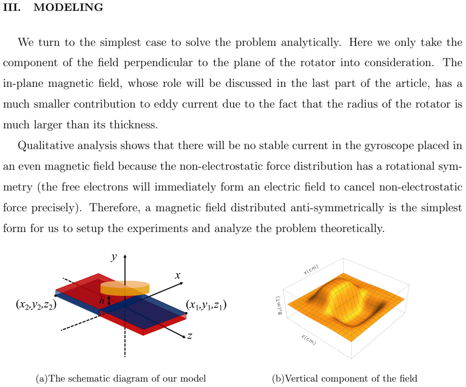
The mechanism carrying the argument is the reduction of Faraday's law plus charge conservation to a Poisson equation for a scalar electric potential $\phi$, with the boundary condition that no current leaves the conductor. Because the rotator is thin and the applied field is taken to have only a $y$ component that depends on the in-plane coordinate $z$, the problem becomes two-dimensional in polar coordinates. Separation of variables through angular eigenfunctions $\phi_n=A_n(r)\cos(n\theta)+B_n(r)\sin(n\theta)$ turns the equation into Euler ordinary differential equations, and the particular-plus-harmonic superposition produces the closed-form currents in Eqs. (30) and (31). The same machinery delivers a torque linear in angular velocity and hence the exponential decay law that is compared with experiment.
What would settle it
Measure the horizontal field component in the rotor plane with a calibrated Hall probe and include its torque in the equation of motion; if the decay-time gap closes from 8.61 percent to near zero, the neglect is confirmed, whereas a sizeable remaining gap would implicate the cubic polynomial fit or the quasi-static assumption.
Extended reading notes
Core claim
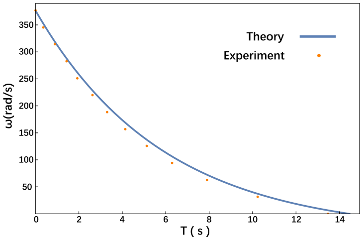
The paper's central claim is that the eddy-current problem in a thin spinning conductor in a static magnetic field can be reduced, without solving the time-dependent Maxwell equations, to the boundary value problem $\nabla^2\phi = \nabla\cdot[(\boldsymbol{\omega}\times\mathbf{r})\times\mathbf{B}]$ with $\mathbf{j}\cdot\hat{\mathbf{n}}=0$ on the surface. Solving this Poisson equation in polar coordinates, by splitting the solution into a particular part and a harmonic part, yields closed-form current densities $\mathbf{j}_1$ and $\mathbf{j}_3$ for the linear and cubic terms of the vertical field. The magnetic torque from these currents is $M=-\lambda\omega$, so the rotational equation $I\,d\omega/dt=-\lambda\omega$ predicts $\omega(t)=\omega_0 e^{-t/\tau}$. After calibrating the magnet remanence and one frictional multiplier, the computed decay time differs from the experiment by 8.61 percent, and the authors trace most of this residual to their neglect of the horizontal field component.
Load-bearing premise
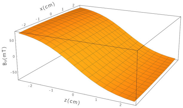
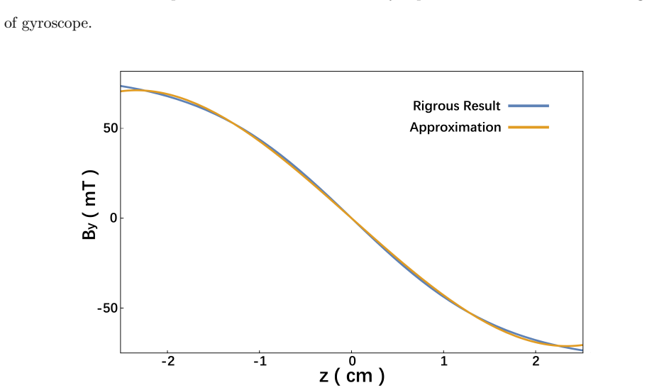
The load-bearing premise is that, in the rotor region, the vertical magnetic field depends only on the in-plane coordinate $z$ and is described by $B_z=k_1 z + k_3 z^3$, while the comparable horizontal field can be neglected; the authors estimate that neglect contributes about 10 percent of the torque, nearly the entire reported 8.61 percent discrepancy.
Editorial extensions
If this is right
- Any static vertical field in the rotor region can be expanded as $k_1 z + k_3 z^3$ or decomposed into symmetric and anti-symmetric parts, so the method transfers to other magnet geometries without numerical simulation.
- The magnetic torque is exactly linear in $\omega$, so the deceleration curve is exponential; this is a sharp prediction that high-precision measurements can confirm or reject.
- The closed-form currents give a quantitative laboratory check for eddy-current demonstrations and a quick estimate of eddy-current losses in thin conducting disks.
- The dominant identified error comes from a single omission, the horizontal field component, so including that component in the torque integral is a direct route toward closing the 8.61 percent gap.
Reading between the lines
- A natural follow-up experiment is to place the magnets so that the cubic term in $B_y$ is negligible, leaving only the linear term; the decay should then be governed entirely by Eq. (30), which would isolate that formula's accuracy.
- The same scalar-potential reduction should extend to other thin rotors such as annular plates or disks of nonuniform thickness, provided the boundary conditions on each edge are imposed separately.
- If the horizontal-field torque were measured or computed independently, the reported 8.61 percent discrepancy should shrink to nearly zero, making the neglect of that component a testable quantitative claim rather than a qualitative error estimate.
Signed reviews
Editorial analysis
A structured set of objections, weighed in public.
Referee Report
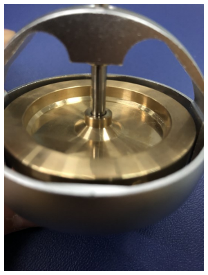
Summary. This manuscript presents an analytical treatment of eddy-current damping in a spinning brass gyroscope. Working in the lab frame and assuming a static magnetic field and quasi-static currents, the authors reduce the problem to a Poisson equation with Neumann boundary conditions, approximate the vertical field component over the rotor as B_z = k1 z + k3 z^3, solve the boundary-value problem for a disk/ring geometry, and obtain closed-form eddy-current expressions. They then compute the magnetic torque as −λω, predict an exponential decay of the rotation frequency, and compare the decay time with strobe-light measurements, reporting a relative error of 8.61%.
Significance. If correct, the paper would offer a compact, pedagogical alternative to series solutions for eddy currents in thin rotating conductors, and the experimental comparison would provide a useful validation. The core quasi-static reduction (Eq. 14) and the divergence calculation in Eq. (25) are standard and check out. However, the printed current formula (30) fails charge conservation as written, the treatment of the composite rotor as independent regions is not physically justified, and the experimental comparison involves calibrated or fitted inputs; these issues currently limit the significance of the paper.
major comments (4)
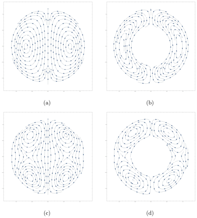
- [Section V, Eq. (30)] The printed θ-component of j1 contains a minus sign in front of a²b²/r². Direct solution of the stated boundary-value problem (25)–(28) gives j1θ = (σωk1/8)(a² + b² + a²b²/r² − 3r²) cosθ, with a plus sign before the a²b²/r² term. With the published minus sign, ∇·j1 = σωk1 a²b²/(4r³) sinθ, which is nonzero wherever a > 0, so Eq. (30) is not a solution of the charge-conserving problem. The radial component appears correct, so the torque may survive a sign correction, but the central claim of a closed-form current distribution is not correct as printed. Eq. (31) should be rechecked with the same divergence test.
- [Section V, Eq. (25) and Fig. 5] The plate and the rings are solved as independent boundary-value problems, each with j_r = 0 at r = a and r = b. If these are parts of a single electrically connected brass rotor, as the description around Fig. 5 suggests, those surfaces are internal conducting interfaces rather than insulating boundaries; the true current distribution must satisfy continuity of the potential and of the normal current across them. The manuscript provides no justification for treating the regions as isolated, so even after correcting Eq. (30), the closed-form currents may not describe the actual assembled rotor. The authors should state whether the regions are electrically isolated or solve the coupled problem.
- [Section VI, Eqs. (32)–(36)] The torque integral leading to τ = 7.839 s is not shown. The paper says 'we can easily calculate' the integral in Eq. (32), but it gives neither an expression for λ nor the integration steps, so the theoretical decay time cannot be reproduced or checked. For a paper whose central quantitative claim is the 8.61% agreement in τ, the derivation of λ as a function of a, b, σ, k1, and k3 should be provided explicitly.
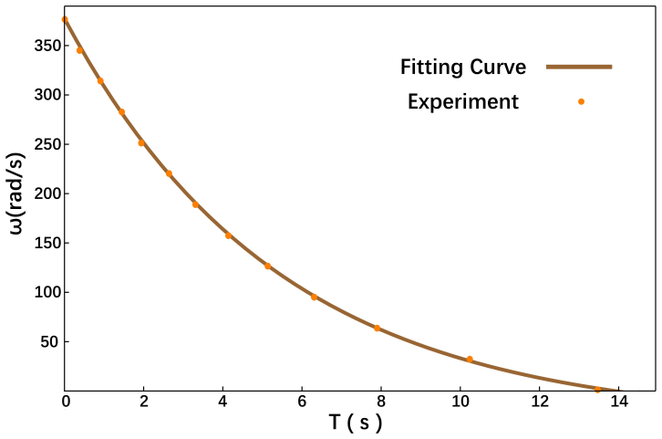
- [Section VI and Section VII] The reported 8.61% agreement is not a parameter-free prediction. In Section IV, Br is described as a fitting parameter and k1, k3 are fitted to the field model; in Section VI, a friction multiplier is fitted so that the theoretical constant term matches the experimental curve. Because the empirical friction torque (36) contains both a constant term M0 and a linear term αω, the fitted multiplier also modifies the effective decay rate (λ + mα)/I, so τ is partly determined by the fit. The paper should state explicitly which quantities are predicted and which are calibrated, and should quantify the sensitivity of τ to the friction multiplier. In addition, the final paragraph of Section VII estimates the neglected in-plane field contribution as about 10% in torque, which is larger than the reported 8.61% discrepancy; this error budget needs a quantitative treatment before the agreement can be interpreted as a validation of the model.
minor comments (6)
- [Eq. (23)] The same vertical component of the magnetic field is denoted both By and Bz in Eq. (23); please fix the coordinate notation so the axes and the field-component subscripts are consistent.
- [Section V] The sentence 'Here we make use of cylindrical coordinates (or polar coordinates since the problem is 2D) them' is ungrammatical and should be rewritten.
- [Section V, Eq. (30)] The radial component of Eq. (30) is written as a sum of two terms; combining them into a single fraction would make it easier to see that the boundary conditions j_r(a) = j_r(b) = 0 are satisfied.
- [Section VI] The text states 'Entering the dimensions and the conductivity of our gyroscope, we get the result that τ = 7.839s' but does not give the conductivity value or the rotor dimensions used in the calculation; please include these inputs.
- [Reference [9]] The title of reference [9] contains a typo: 'Three-Dimentional' should be 'Three-Dimensional'.
- [Fig. 6 caption] The phrase 'top-down anti-symmetry' is unclear; presumably 'top-bottom anti-symmetry' is intended.
Circularity Check
No significant circularity: the eddy-current derivation is self-contained and the reported comparison is a calibrated-model validation, not a construction-level reduction to its inputs.
full rationale
The paper derives the eddy-current boundary value problem from Maxwell's equations, Ohm's law, and charge conservation, then solves the resulting Poisson equation in the rotor geometry. The magnetic field enters as an external input via the Schlueter-Marks magnetostatic formula, with the remanence Br and the polynomial coefficients k1, k3 treated as calibrated/fitted auxiliary parameters; these are not defined in terms of the predicted decay time. The frictional torque multiplier is fitted so that the constant offset in the theoretical decay curve matches the experimental offset, but the reported characteristic decay time τ is a separate output of the same differential equation, so the 8.61% comparison is a genuine one-parameter calibration followed by a prediction of a different observable, not a prediction forced by construction. There are no load-bearing self-citations, no imported uniqueness theorems, and no ansatz smuggled in via citation. The possible charge-conservation violation in Equation (30) and the separate treatment of disk and ring regions are mathematical/physical correctness issues, not circularity, and therefore do not raise the circularity score.
Assumptions & free parameters
free parameters (4)
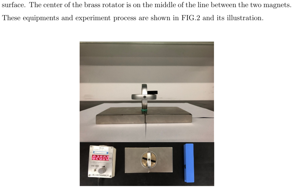
- Br (magnet remanence) =
about 600 mT (calibrated)
- k1 =
-45.67 mT/cm
- k3 =
2.785 mT/cm^3
- friction multiplier m =
not stated
assumptions (7)
- standard math Maxwell equations and Ohm's law, j = σ(E + f)
- domain assumption Quasi-static approximation: ∂ρ/∂t = 0 and displacement current neglected
- domain assumption Magnetic field produced by eddy currents is negligible
- domain assumption Motional emf is f = (ω×r)×B and the magnetic force does not affect the current distribution
- ad hoc to paper The vertical magnetic field over the rotor is a function of the in-plane coordinate z only and is approximated by Bz = k1 z + k3 z^3
- domain assumption Magnetostatic field model uses μr = 1 for the permanent magnets
- domain assumption Rotor is thin enough that the problem is translationally invariant along y and the horizontal field can be neglected
Cite this review
Pith. "Pith review of An Analytical Approach to Eddy Current in Electromagnetic Damping." pith.science (2026). https://pith.science/paper/NVEQFYBH
@misc{pith2026190804713,
  author       = {Pith},
  title        = {Pith review of: An Analytical Approach to Eddy Current in Electromagnetic Damping},
  year         = {2026},
  howpublished = {\url{https://pith.science/paper/NVEQFYBH}},
  note         = {Machine review of arXiv:1908.04713}
}
read the original abstract
An analytical method of calculating eddy current in a metallic spinning gyroscope in external magnetic field is presented. With reasonable assumptions, the problem is simplified from the time-dependent one governed by Maxwell equations to the boundary value problem of Poisson equation, which yields a closed form expression of the eddy current. The rotation frequency as a function of time is calculated, compared with experiment and the relative error is found to be 8.61%.
Figures
Figures from the paper (5 more)
Reference graph
Works this paper leans on
-
[1]
The current varies so slowly with time that it can be treated as nearly time-independent, which means ∂ρ/∂t = 0
-
[2]
The non-electrostatic force here is due to the rotation of the gyroscope, which can be expressed as: ⃗f =⃗ vrot× ⃗B = (⃗ ω×⃗ r)× ⃗B, (13) where⃗ vrot represents the velocity of a particular point on the rotator, ⃗ ωis the angular velocity of the rotator and ⃗ ris the position vector from the center of the gyroscope
-
[3]
The magnetic field supplies the current, and this force acts on the gyroscope directly causing its rotation slow down, but does not affect current distribution. With these assumptions, we can use a much more concise Poisson’s Equation to calculate the current in the gyroscope: ∇2ϕ = ⃗∇· [(⃗ ω×⃗ r)× ⃗B]. (14) We then calculate the deceleration process by eva...
-
[4]
Problems for 32nd IYPT 2019: 12. Gyroscope Teslameter. https://iypt.org/index.php/ problems/problems-for-the-32nd-iypt-2019/
work page 2019
-
[5]
Magnet / Gyroscope MYSTERY! Solve this unseen video
Youtube video: VIDEO 111 UNCOVERING SECRETS OF MAGNETISM. Magnet / Gyroscope MYSTERY! Solve this unseen video. https://www.youtube.com/watch?v= 1ZeCIejT2NY
-
[6]
Richard P. Feynman, Robert B. Leighton, and Matthew Sands, The Feynman Lectures on Physics, Vol. 2 (Addison-Wesley, 1964), p. 17-2
work page 1964
-
[7]
On Eddy Currents in a Rotating Disk
W. R. Smythe, “On Eddy Currents in a Rotating Disk”, Electrical Engineering, Vol. 61, p. 681, 1942
work page 1942
-
[8]
Braking torque on rotating sheet in stationary magnetic field
D. Schieber, “Braking torque on rotating sheet in stationary magnetic field”, Proceedings of the Institution of Electrical Engineers, Vol. 121, No.2, p. 117, 1974
work page 1974
Show all 15 references
-
[9]
Drag and lift forces between a rotating conductive sphere and a cylindrical magnet
M. A. Nurge, R. C. Youngquist, and S. O. Starr, “Drag and lift forces between a rotating conductive sphere and a cylindrical magnet ” American Journal of Physics, Vol. 86(6), p. 443, 2018
2018
-
[10]
Feynman, Robert B
Richard P. Feynman, Robert B. Leighton, and Matthew Sands, The Feynman Lectures on Physics, Vol. 2 (Addison-Wesley, 1964), p. 2-1
1964
-
[11]
Griffiths, Introduction to Electrodynamics, 3rd edition (Prentice Hall, 1999), p
David J. Griffiths, Introduction to Electrodynamics, 3rd edition (Prentice Hall, 1999), p. 285– 301
1999
-
[12]
Three-Dimentional Pure Permanent Magnet Undulator Design Theory
R. D. Schlueter and S. Marks, “Three-Dimentional Pure Permanent Magnet Undulator Design Theory”, IEEE Transactions on Magnetics, Vol. 32, No. 4
-
[13]
Design of permanent multiple magnets with oriented rare earth cobalt material
K. Halbach, “Design of permanent multiple magnets with oriented rare earth cobalt material”, 19 Nucl. Instr. Meth. vol. 169, p. 1, 1980
1980
-
[14]
Physical and optical properties of rare earth cobalt magnets
K. Halbach, “Physical and optical properties of rare earth cobalt magnets”, Nucl. Instr. Meth. vol. 187, p. 109, 1981
1981
-
[15]
Shengshan Cai, Yun Zhu, Jianjun Xu, Electrodynamics, 2rd edition (Higher Education Press, 2005), p. 142 20
2005
Reviewed August 14, 2026 · model on record in the stance chip above.
Discussion (0). Continue with ORCID to comment.