REVIEW 4 major objections 5 minor 26 references
On Multivariate Financial Time Series Classification
T0 review · 4 major / 5 minor · reviewed 2026-08-16 · deepseek-v4-flash
Pith's one-line read This paper argues that large multivariate financial datasets favor fully convolutional deep classifiers over classical models, reporting a 20% EUR/USD strategy return on flat markets.
desk verdict A survey with an invalid key experiment: the 20% return is an in-sample artifact, so the paper's central claim collapses, though the exposition has some pedagogical value. read the letter →
The pith
A machine-rendered reading of the paper's core claim, the machinery that carries it, and where it could break.
The reading
What carries the argument
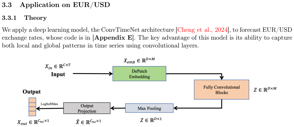
The central mechanism is a three-class labeling scheme combined with a fully convolutional deep network. Returns are shifted and split at the 33rd and 67th percentiles into -1, 0, +1 classes; the network, implemented in Appendix E as a two-block 1D CNN with batch normalization, ReLU, adaptive average pooling, dropout, and a linear head, is trained with cross-entropy loss and the Adam optimizer. Strategy returns multiply the predicted signal by the realized return and are accumulated to produce the comparison curves against market and random strategies. The text describes the model as ConvTimeNet, with deformable patch embedding and fully convolutional blocks, and stresses the O(n·k) complexity of convolutions versus O($n^{2}$) attention as the scaling advantage.
What would settle it
Train ConvTimeNet on the first 80,000 minute-level EUR/USD samples and freeze the model, then compute strategy returns on the last 20,000 samples; if the 20% excess return shrinks to the random or market baseline, the paper's claim that the model identifies exploitable patterns is unsupported.
Extended reading notes
Core claim
The paper's central claim is that the right tool for financial time series classification shifts with data scale: on small datasets, classical models such as SVMs and XGBoost can appear to beat the market but are really overfitting, while on big datasets a fully convolutional network can capture exploitable structure. Applying a ConvTimeNet-style architecture to 100,000 minute-level EUR/USD samples with 200 features, the author reports a cumulative strategy return of 20% while the market stays flat, and takes this as evidence that the model found profitable short-term patterns. The paper also reports that in the small-data regime, final cumulative returns deteriorate as the number of observations grows from 500 to about 1,700, which it reads as a decreasing signal-to-noise ratio rather than a reason to prefer more data.
Load-bearing premise
The headline result assumes that computing trading returns from predictions on the training set says something about future performance, since the model is trained and evaluated on the same 100,000 samples.
Editorial extensions
If this is right
- Big-data convolutional classifiers can in principle generate positive strategy returns on minute-level FX data even when the underlying market is flat, which is the paper's main evidence for learnable structure.
- Small-data financial backtests should be regarded as overfit unless validated on data the model has not seen, because the same workflow that looks strong on Strike fails on Bitcoin.
- Convolutional architectures scale better than attention-based ones for high-frequency multivariate series, making them a practical choice as data volume grows.
- More observations do not automatically improve classification accuracy; in the small-data experiments, performance falls as the sample grows, suggesting signal quality matters as much as quantity.
Reading between the lines
- Appendix E trains on all 100,000 EUR/USD samples and then computes the strategy return on the same samples, so the 20% figure is an in-sample statistic; the paper does not report a temporal holdout, and that is the test that would turn the claim into evidence of out-of-sample skill.
- The random-strategy comparison is a single random draw; averaging many random seeds would show whether the model's edge is wider than the noise of random trading.
- Because the 33rd and 67th percentile thresholds are computed on the full dataset, the labels may embed future information; computing the thresholds in a rolling or walk-forward manner would be a direct robustness check.
- The Appendix E code implements a simple two-convolution network rather than the deformable-patch ConvTimeNet described in the text, so the reported result should be attributed to the implemented architecture.
Signed reviews
Editorial analysis
A structured set of objections, weighed in public.
Referee Report
Summary. The manuscript compares small-data and big-data machine learning approaches for multivariate financial time series classification, using EUR/USD and cryptocurrency datasets. It describes traditional models (XGBoost, SVM, LSTM) and a deep learning model attributed to ConvTimeNet, and reports trading-simulation results in terms of cumulative returns against market and random strategies. The headline result is a 20% cumulative return in Section 3.3.2 from a ConvTimeNet-style model trained on 100,000 minute-level EUR/USD samples. The paper concludes that big data can be beneficial for identifying profitable patterns, though it also discusses overfitting in small data and market adaptation.
Significance. If the 20% out-of-sample return were valid, the paper would offer a noteworthy demonstration that convolutional models can extract tradeable signals from high-frequency FX data. The paper is transparent in providing full code appendices, which allow the evaluation protocol to be checked directly. However, the central empirical claim is not established, because the reported performance is computed on the training set; the significance of the contribution therefore rests on an evaluation that provides no out-of-sample evidence.
major comments (4)
- [§3.3.2, Appendix E] The headline 20% cumulative return is computed on the same data used for training. Appendix E line 22 defines df_min as the first 100,000 samples; line 30 fits the StandardScaler on this full set; line 38 creates a DataLoader for the full dataset; lines 68–76 train the model for 100 epochs on this dataset; line 91 computes predictions on the same DataLoader; and lines 94–101 derive strategy returns and cumulative returns from those predictions. There is no train/test split, temporal holdout, or walk-forward validation. The claim in Section 3.3.2 that the model 'was able to identify profitable patterns in the EUR/USD data' is therefore unsupported; the 20% figure reflects in-sample training accuracy, not predictive skill.
- [§2.3.2, Appendix B] The small-data experiments use the same in-sample evaluation: after hyperparameter selection with TimeSeriesSplit, Appendix B line 108 calls best_model.predict(features_scaled) on the full feature set, and line 110 forms strategy returns on the same data. Consequently, Figure 13 and the small-data backtests in Figures 6 and 7 are based on training-set predictions. The paper explicitly acknowledges in Section 2.3.2 that the small-data outperformance 'is often the result of overfitting,' but the identical protocol flaw is not controlled in the big-data experiment, so the claimed contrast between small and big data is not established.
- [Appendix E, lines 40–60] The implemented network does not correspond to the ConvTimeNet architecture described in Section 3.2.1 and cited to [Cheng et al., 2024]. The code defines a plain two-layer 1D CNN with batch normalization and adaptive average pooling; it contains no deformable patch embedding and no fully convolutional blocks with deepwise and pointwise convolutions. Thus the experiments evaluate a generic CNN baseline, not the architecture named in the paper, and any results cannot be attributed to ConvTimeNet.
- [§3.3.2, Appendix E line 96] The comparison against a random strategy is based on a single random draw of signals with no repetitions, error bars, or significance test. Given the high noise level of minute-level FX returns, the observed difference between the model and one random realization could arise by chance; the manuscript provides no statistical evidence that the model's performance exceeds a random baseline.
minor comments (5)
- [§1.1.1] The GARCH model is cited to [Engle and Ng, 1982]; the standard reference for GARCH is Engle (1982), and the authors may want to correct the citation.
- [§2.3.2, Figure 13] Figure 13 is referenced in the text but its construction is described only through code in Appendix B; the text should state the dataset sizes and models shown.
- [§3.3.1] The data source for the EUR/USD dataset is not described in the main text; the paper should state the provider, period, and feature definitions.
- [Appendices A and E] The random strategy in Appendix A uses choices {0,1} while Appendix E uses {-1,0,1}; the difference should be explained or reconciled.
- [Appendix E] The code listing contains several corrupted imports and repeated lines; a clean, executable version of the appendices would improve reproducibility.
Circularity Check
The 20% return in Section 3.3.2 is computed on the same 100,000 samples used for training (Appendix E), so the headline prediction reduces to in-sample fit.
-
fitted input called prediction
[Section 3.3.2 Results and Appendix E, lines 22, 30, 38, 67–76, 91–102]
"Appendix E: "df_min = df . iloc [:100 _000 ]" ... "dataloader = DataLoader ( dataset , b a t c h _ s i z e =32 , shuffle = True )" ... "for epoch in range ( epochs ) : ... optimizer . step ()" ... "predicted_signals = predict ( model , dataloader )". Section 3.3.2: "As shown in the results, the model outperformed the random strategy, generating a final return of 20% while the market remained relatively flat. This indicates that the model was able to identify profitable patterns in the EUR/USD data.""
The evaluation protocol has no train/test split: line 22 selects the full 100,000 samples, line 30 fits the StandardScaler on all of them, line 38 builds a DataLoader over the full dataset with shuffle=True, lines 67–76 train the model for 100 epochs on that same DataLoader, and line 91 computes predictions on the same DataLoader. The strategy returns (line 94) and cumulative returns (lines 99–102) are therefore computed from predictions on the training data. A flexible convolutional network trained for 100 epochs can fit the training labels, so the reported 20% final return is an in-sample fit statistic, not an out-of-sample prediction. The headline claim that the model "identified profitable patterns" thus reduces by construction to training-set fit quality.
full rationale
The paper's theoretical exposition in Sections 1 through 3.2 is standard survey material and is not circular. The only load-bearing empirical claim is the Section 3.3.2 result, and Appendix E shows that the ConvTimeNet model was trained and evaluated on the identical 100,000-sample dataset: the scaler is fit on all data, the DataLoader covers the full dataset, the model is trained for 100 epochs on that loader, and predictions are then generated from the same loader. Because there is no temporal holdout or walk-forward validation, the reported 20% return and the conclusion that the model identified profitable patterns are in-sample training performance, not predictions. The percentile-based target construction in Section 2.3.2 is also computed from the full dataset, which compounds the leakage, though the decisive circularity is scoring on the training set. No self-citation chain, uniqueness theorem, or ansatz-smuggling via citation appears, so a score of 6 reflects partial circularity: the central result reduces by construction to a training fit.
Assumptions & free parameters
free parameters (3)
- label thresholds =
Q0.33 and Q0.67 of the return distribution
- model hyperparameters =
grid search results (e.g., C, gamma, n_estimators)
- ConvTimeNet architecture =
kernel size 3, channels 64/128, dropout 0.5
assumptions (3)
- domain assumption Historical price features contain predictive information for future returns
- domain assumption The 200-feature feature matrix is sufficient and correctly preprocessed
- domain assumption Sequential splits and in-sample scoring provide unbiased performance estimates
Cite this review
Pith. "Pith review of On Multivariate Financial Time Series Classification." pith.science (2026). https://pith.science/paper/O4JXYOEP
@misc{pith2026250417664,
  author       = {Pith},
  title        = {Pith review of: On Multivariate Financial Time Series Classification},
  year         = {2026},
  howpublished = {\url{https://pith.science/paper/O4JXYOEP}},
  note         = {Machine review of arXiv:2504.17664}
}
read the original abstract
This article investigates the use of Machine Learning and Deep Learning models in multivariate time series analysis within financial markets. It compares small and big data approaches, focusing on their distinct challenges and the benefits of scaling. Traditional methods such as SVMs are contrasted with modern architectures like ConvTimeNet. The results show the importance of using and understanding Big Data in depth in the analysis and prediction of financial time series.
Figures


Figures from the paper (13 more)



Reference graph
Works this paper leans on
-
[1]
Abe, S. and Abe, S. (2010). Feature selection and extraction. Support vector machines for pattern classification , pages 331--341
work page 2010
-
[2]
A., Sarker, Y., Chakrabortty, R
Asif, N. A., Sarker, Y., Chakrabortty, R. K., Ryan, M. J., Ahamed, M. H., Saha, D. K., Badal, F. R., Das, S. K., Ali, M. F., Moyeen, S. I., et al. (2021). Graph neural network: A comprehensive review on non-euclidean space. Ieee Access , 9:60588--60606
work page 2021
-
[3]
Cheng, M., Yang, J., Pan, T., Liu, Q., and Li, Z. (2024). Convtimenet: A deep hierarchical fully convolutional model for multivariate time series analysis. arXiv preprint arXiv:2403.01493
work page Pith review arXiv 2024
-
[4]
Christ, M., Kempa-Liehr, A. W., and Feindt, M. (2016). Distributed and parallel time series feature extraction for industrial big data applications. arXiv preprint arXiv:1610.07717
arXiv 2016
-
[5]
Cortes, C. (1995). Support-vector networks. Machine Learning
work page 1995
-
[6]
Dixon, M., Klabjan, D., and Bang, J. H. (2017). Classification-based financial markets prediction using deep neural networks. Algorithmic Finance , 6(3-4):67--77
work page 2017
-
[7]
Engle, R. F. and Ng, V. (1982). An introduction to the use of arch/garch models in applied econometrics. Journal of Business, New York
work page 1982
-
[8]
Fons, E., Dawson, P., Zeng, X.-j., Keane, J., and Iosifidis, A. (2020). Evaluating data augmentation for financial time series classification. arXiv preprint arXiv:2010.15111
arXiv 2020
Show all 26 references
-
[9]
Fukushima, K. (1969). Visual feature extraction by a multilayered network of analog threshold elements. IEEE Transactions on Systems Science and Cybernetics , 5(4):322--333
1969
-
[10]
and Qi, M
Gen c ay, R. and Qi, M. (2001). Pricing and hedging derivative securities with neural networks: Bayesian regularization, early stopping, and bagging. IEEE transactions on neural networks , 12(4):726--734
2001
-
[11]
S., and Ye, M
Goldstein, I., Spatt, C. S., and Ye, M. (2021). Big data in finance. The Review of Financial Studies , 34(7):3213--3225
2021
-
[12]
C.-I., and Si, Y.-W
He, Q.-Q., Pang, P. C.-I., and Si, Y.-W. (2019). Transfer learning for financial time series forecasting. In PRICAI 2019: Trends in Artificial Intelligence: 16th Pacific Rim International Conference on Artificial Intelligence, Cuvu, Yanuca Island, Fiji, August 26--30, 2019, Pr...
2019
-
[13]
A., Dumais, S
Hearst, M. A., Dumais, S. T., Osuna, E., Platt, J., and Scholkopf, B. (1998). Support vector machines. IEEE Intelligent Systems and their applications , 13(4):18--28
1998
-
[14]
Hochreiter, S. (1997). Long short-term memory. Neural Computation MIT-Press
1997
-
[15]
Ismail Fawaz, H., Forestier, G., Weber, J., Idoumghar, L., and Muller, P.-A. (2019). Deep learning for time series classification: a review. Data mining and knowledge discovery , 33(4):917--963
2019
-
[16]
Krešňáková, V., Sarnovsky, M., Butka, P., and Machova, K. (2020). Comparison of deep learning models and various text pre-processing techniques for the toxic comments classification. Applied Sciences , 10:8631
2020
-
[17]
Kumar, A., Kiran, M., and Prathap, B. (2013). Verification and validation of mapreduce program model for parallel k-means algorithm on hadoop cluster. In 2013 Fourth International Conference on Computing, Communications and Networking Technologies (ICCCNT) , pages 1--8. IEEE
2013
-
[18]
Kwak, N. (2013). Nonlinear projection trick in kernel methods: An alternative to the kernel trick. IEEE transactions on neural networks and learning systems , 24(12):2113--2119
2013
-
[19]
Lemley, J., Bazrafkan, S., and Corcoran, P. (2017). Transfer learning of temporal information for driver action classification
2017
-
[20]
Lo, A. W. (2004). The adaptive markets hypothesis: Market efficiency from an evolutionary perspective. Journal of Portfolio Management, Forthcoming
2004
-
[21]
Lunga, D., Gerrand, J., Yang, L., Layton, C., and Stewart, R. (2020). Apache spark accelerated deep learning inference for large scale satellite image analytics. IEEE Journal of Selected Topics in Applied Earth Observations and Remote Sensing , 13:271--283
2020
-
[22]
E., Hinton, G
Rumelhart, D. E., Hinton, G. E., and Williams, R. J. (1986). Learning internal representations by error propagation, parallel distributed processing, explorations in the microstructure of cognition, ed. de rumelhart and j. mcclelland. vol. 1. 1986. Biometrika , 71(599-607):6
1986
-
[23]
A., Cenedese, A., and Terzi, M
Susto, G. A., Cenedese, A., and Terzi, M. (2018). Time-series classification methods: Review and applications to power systems data. Big data application in power systems , pages 179--220
2018
-
[24]
Wang, Y., Huang, M., Zhu, X., and Zhao, L. (2016). Attention-based lstm for aspect-level sentiment classification. In Proceedings of the 2016 conference on empirical methods in natural language processing , pages 606--615
2016
-
[25]
Wu, D., Wang, X., Su, J., Tang, B., and Wu, S. (2020). A labeling method for financial time series prediction based on trends. Entropy , 22(10):1162
2020
-
[26]
Yin, J., Rao, W., Yuan, M., Zeng, J., Zhao, K., Zhang, C., Li, J., and Zhao, Q. (2019). Experimental study of multivariate time series forecasting models. In Proceedings of the 28th ACM international conference on information and knowledge management , pages 2833--2839
2019
Reviewed August 16, 2026 · model on record in the stance chip above.
Discussion (0). Continue with ORCID to comment.