REVIEW 4 major objections 8 minor 45 references
Locate a stellar flare from the M dwarf LAMOST J1332+5057
T0 review · 4 major / 8 minor · reviewed 2026-07-31 · grok-4.5
Pith's one-line read A young M dwarf's flare is located near the pole using Mg I b radial velocities from eight LAMOST spectra.
desk verdict Real high-latitude signal from Mg I b RVs, but the quoted polar coordinate rests on the last three fading exposures and an untested constant-v⊥ assumption. read the letter →
The pith
A machine-rendered reading of the paper's core claim, the machinery that carries it, and where it could break.
The reading
What carries the argument
The projected-velocity model v(t) = Ve sini · cos θ0 · sin(φ0 + 2π t/Prot) − v⊥ [sin i cos θ0 cos(φ0 + 2π t/Prot) + sin θ0 cos i] + RV, fitted by MCMC to the eight Mg I b centroid velocities; the small observed Δv forces high |θ0|.
What would settle it
A second multi-epoch spectroscopic campaign on the same star (or a twin) that yields a clearly larger Mg I b velocity swing during another flare of similar energy would force a lower latitude and break the polar placement.
Extended reading notes
Core claim
Using the time series of Mg I b radial velocities measured in eight continuous LAMOST medium-resolution exposures of a white-light flare on the young M dwarf J1332+5057, the authors invert a simple geometric model and locate the flare at (φ0, θ0) = (−123.0^{+8.0}_{-5.8}, 80.5^{+2.9}_{-3.2}) degrees, i.e., in the polar region.
Load-bearing premise
The Mg I b light is assumed to come from one compact, fixed surface patch whose vertical flow stays constant for the whole 2.9-hour sequence; if the emitting region is extended or evolving, the latitude-longitude solution is biased.
Editorial extensions
If this is right
- High-latitude flares on fast-rotating M dwarfs would deliver a lower average CME and particle dose to planets near the ecliptic than equatorial flares of the same energy.
- The same Mg I b velocity time series can be applied to other LAMOST or high-resolution flare spectra to build a statistical map of flare latitudes.
- Polar flare sites would support the theoretical expectation that rapid rotation drives magnetic flux tubes to high latitudes.
- Angular-momentum loss and space-weather models for young M dwarfs must incorporate latitude-dependent CME deflection rather than assume solar-like equatorial belts.
Reading between the lines
- If Mg I b remains the cleanest tracer, coordinated multi-site spectroscopy of a single flare could resolve whether the emitting patch itself drifts in latitude as the flare decays.
- The method is naturally complementary to continuum light-curve modeling of flare asymmetry; joint fits would test whether white-light and Mg I b centroids coincide.
- A larger sample of polar versus equatorial flares on stars of known Rossby number would directly constrain how the dynamo’s preferred emergence latitude scales with rotation.
Editorial analysis
A structured set of objections, weighed in public.
Referee Report
Summary. The authors identify a 2.89-hour, eight-exposure LAMOST MRS spectral sequence of a white-light flare on the young, rapidly rotating (Prot = 0.423 d, Ve sin i = 35 km/s) M dwarf J1332+5057. After subtracting a scaled quiescent template and a parabolic flare continuum, they fit the Mg I b λ5174/λ5185 emission lines with tied Gaussians and measure radial-velocity centroids (Table 2) that drift from −9.7 to −6.1 km/s over the sequence. Modeling the centroid as the sum of projected rotation of a surface-fixed site plus a constant vertical flow v⊥ (Eqs. 19–21), an MCMC fit with stellar priors yields a flare location of (φ0, θ0) = (−123.0°, 80.5°), i.e. polar. A model-independent bound in Appendix B (θ0 ≳ 79.7°) supports the high latitude within the model's assumptions. The work would, if robust, provide the first spectroscopic kinematic localization of a stellar flare and a reusable method.
Significance. If the interpretation holds, this is the first spectroscopic radial-velocity localization of a stellar flare, and the first at polar latitude derived from line kinematics rather than light-curve modeling. Notable strengths: Appendix B provides a genuinely useful model-light bound (θ0 ≳ 79.7°) requiring only Ve sin i, two velocity measurements, and the period; the stellar priors come from independent data (APOGEE, Gaia, TESS), so the inference is not circular; the MCMC machinery is standard (emcee) with reported convergence diagnostics; and the flare-only spectra are publicly released, making the analysis reproducible. The method is cheap and directly applicable to the large LAMOST MRS archive, with clear relevance to CME–planet impact geometry and to dynamo models of rapid rotators. The result is also falsifiable in principle via repeat flares from the same active longitude.
major comments (4)
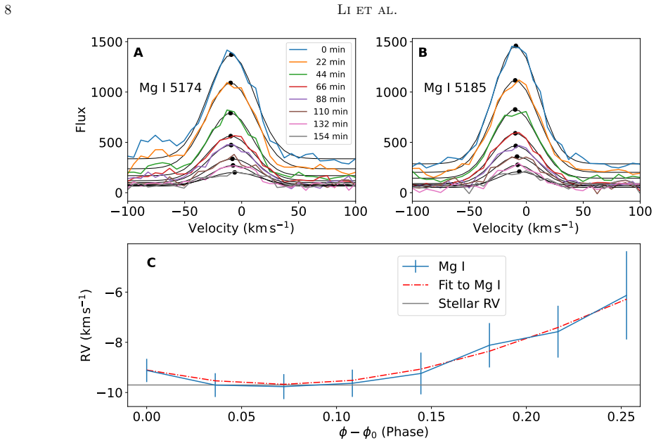
- [§5, Eqs. (17)–(21); Appendix B; Table 2] Constant-v⊥, single-site assumption (Eqs. 17–21; App. B16–B23): this premise is load-bearing and untested. Per Table 2, exposures 1–5 are flat (−9.1 to −9.7 km/s, σ≈0.5) and the entire 3.6 km/s drift occurs in exposures 6–8, where the fading line's centroid errors grow to ±0.9, ±1.0, ±1.8. An evolving vertical flow (chromospheric condensation downflows decay on tens of minutes) or a flux-weighted centroid of a rotating kernel plus a decaying flow component would mimic this drift; Eq. 21's likelihood would then attribute intrinsic evolution to geometry, and the App. B bound, which requires constant v⊥ between t1 and t2, would not apply. The claim in §4 that Mg I b is 'stable' addresses line width, not centroid. Required: (i) fit an explicit time-varying v⊥(t) alternative and compare model evidence; (ii) a leave-one-out test on each of the last three exposures; (iii) demonstration that θ0≳
- [§4, Eqs. (17)–(18), Fig. 5; §5, Eq. (22)] No goodness-of-fit or residual analysis is reported for either the per-exposure double-Gaussian fits or the global MCMC fit of Eq. (21) to 8 velocities with 3 flare parameters plus priors. Please report χ²/dof and show a residuals panel for Fig. 5C. Additionally, the Fe I λ5173 bump on the blue wing of Mg I λ5174 (visible in Fig. 5A) is absorbed into a single-Gaussian-plus-constant model; if the Fe I/Mg I flux ratio varies through the flare, the blend biases the fitted vc. Quantify this bias per exposure, e.g. by fitting a third component or masking the blend region, and propagate it into Table 2.
- [§5, Eqs. (19)–(21); Fig. 9] The model v(t) is invariant under (θ0, v⊥) → (−θ0, −v⊥): v1 depends on cosθ0 and the constant term on the product v⊥sinθ0. The flare hemisphere is therefore formally degenerate, and v⊥ is degenerate in sign with it. The paper does not discuss this; Fig. 9 shows only positive θ0. Please state the hemisphere ambiguity explicitly, describe the prior/posterior handling (was θ0 bounded to [0,90°]?), and confirm the quoted errors are not artifacts of a truncated posterior.
- [§2, Eqs. (3)–(6); Appendix B (B16)–(B23)] Quiescent subtraction: Eq. (3) assumes fQ = a·fQ,0 with a single scalar scaling of a spectrum taken on a different night, plus a parabolic flare continuum, and Eq. (6) neglects covariance between (a,b,c,d) and the pixel errors. Template mismatch or chromospheric variability residuals near 5174/5185 Å could shift centroids at the km/s level — comparable to the 3.6 km/s signal. Please show the flare-only residuals around the Mg I b region for all eight exposures and estimate the resulting centroid uncertainty. Related: the App. B bound requires the two velocities to lie 'in the same monotonic interval' (B16–B18); with 8 points over 0.25 of a rotation, how is this established for t=44 and t=154 min without already assuming the fitted φ0? Please clarify.
minor comments (8)
- Typos: §3.1 'template liberary'; §5 'dfference'; Fig. 6 'light of sight' should be 'line of sight'. Abstract: 'would seriously impact' → 'can seriously impact'.
- Abstract and Conclusion: 'pinpointed' and 'accurately locate' overstate a single-flare, model-dependent result; suggest 'localized, under the stated single-site assumptions'.
- §5 text reports θ0 = 80.5^{+3.0}_{−3.2} while the abstract and preceding sentence give 80.5^{+2.9}_{−3.2}; unify.
- State the sign convention of v⊥: the fitted −7.5±2.3 km/s presumably denotes downflow; a sentence on its physical plausibility relative to chromospheric condensation velocities would strengthen the paper.
- Table 2: add per-exposure S/N or Mg I equivalent width so the reader can see directly why the last three errors grow; this is central to interpreting the drift.
- Fig. 4B: the claim that Mg I b is 'stable' while Hα varies should be quantified (e.g., EW and width versus time) rather than shown only as normalized profiles.
- Eq. (13): note how MCMC samples with Ve sin i > Ve (unphysical i) are handled in emcee.
- Consider citing Doppler/Zeeman–Doppler imaging work on polar spots in rapid rotators as independent context for high-latitude magnetic activity.
Circularity Check
No circularity: flare coordinates are free parameters fitted to independent Mg I b RV time series via an explicit geometric projection, not defined by or forced from the inputs.
full rationale
The load-bearing chain is: (1) flare-only spectra via scaled quiescence + parabola continuum (Eqs. 3–5); (2) Gaussian centroids of Mg I λ5174/5185 giving eight measured RVs (Table 2, Eqs. 17–18); (3) geometric model v(t)=v_rot(φ0,θ0,t)+v⊥_proj(φ0,θ0,t)+RV (Eqs. 19–21); (4) MCMC posterior on (φ0,θ0,v⊥) with external stellar priors (Teff, ϖ, Prot, RV, Ve sin i from APOGEE/Gaia/TESS/templates). The reported location (−123°, 80.5°) is the fitted output of that likelihood, not a quantity defined in terms of itself, nor a ‘prediction’ of a closely related fitted input. The App. B lower bound θ0≳79.7° is a direct algebraic consequence of the same projection under constant-v⊥ and same-monotonic-interval assumptions; it does not smuggle the answer. Self-citations (Li et al. 2023/2024) support only ancillary TESS flare detection/FFD context and are not load-bearing for (φ0,θ0). Concerns that Δv may be intrinsic flare-decay flow rather than rotation are model-validity/assumption issues, not circularity. The derivation is self-contained against its stated inputs.
Assumptions & free parameters
free parameters (6)
- flare longitude φ0 =
−123.0^{+8.0}_{-5.8} deg
- flare latitude θ0 =
80.5^{+2.9}_{-3.2} deg
- vertical chromospheric velocity v⊥ =
−7.5±2.3 km s−1
- per-spectrum continuum/scale coefficients a,b,c,d
- Gaussian amplitudes, widths, and baselines for Mg I λ5174 and λ5185
- linear limb-darkening coefficient ε =
0.8 (fixed)
assumptions (6)
- domain assumption Mg I b emission in the flare forms in a cool chromospheric region that can be treated as a single surface site with one radial velocity, analogous to solar Mg I behavior (Sasso et al. 2017).
- ad hoc to paper Flare continuum under the lines is a low-order parabola and the true quiescence during the flare night equals a constant times the May 8 coadded spectrum.
- domain assumption Projected rotational velocity of a surface element follows the standard rigid-rotation Doppler formula with known i and Ve (Gray-type kernel).
- ad hoc to paper Net vertical velocity v⊥ is constant in time and uniform over the emitting site during the 2.89 h sequence.
- domain assumption The two Mg I lines share one centroid velocity each epoch and are adequately described by single Gaussians (Fe I blend on λ5174 treated as a wing bump).
- domain assumption Stellar Prot, Ve sin i, RV, and inclination priors from TESS/APOGEE/Gaia/PHOENIX are accurate enough that residual systematics are smaller than the flare Δv signal.
Cite this review
Pith. "Pith review of Locate a stellar flare from the M dwarf LAMOST J1332+5057." pith.science (2026). https://pith.science/paper/OGDFLEDN
@misc{pith2026260724284,
  author       = {Pith},
  title        = {Pith review of: Locate a stellar flare from the M dwarf LAMOST J1332+5057},
  year         = {2026},
  howpublished = {\url{https://pith.science/paper/OGDFLEDN}},
  note         = {Machine review of arXiv:2607.24284}
}
abstract
Young M-type stars exhibit frequent flares, which would seriously impact their habitable planets. Since stellar surfaces cannot be resolved, flare locations remain unknown. Here, by using the Mg I b emission line in LAMOST spectra, the location of a stellar flare from a young M dwarf is pinpointed at $ (-123.0^{+8.0}_{-5.8}, 80.5^{+2.9}_{-3.2})$ in degree in the polar region. Our method can be used to accurately locate stellar flares. This would enable us to assess the impact of stellar flares on planets more accurately and improve our understanding of stellar dynamo models.
Figures
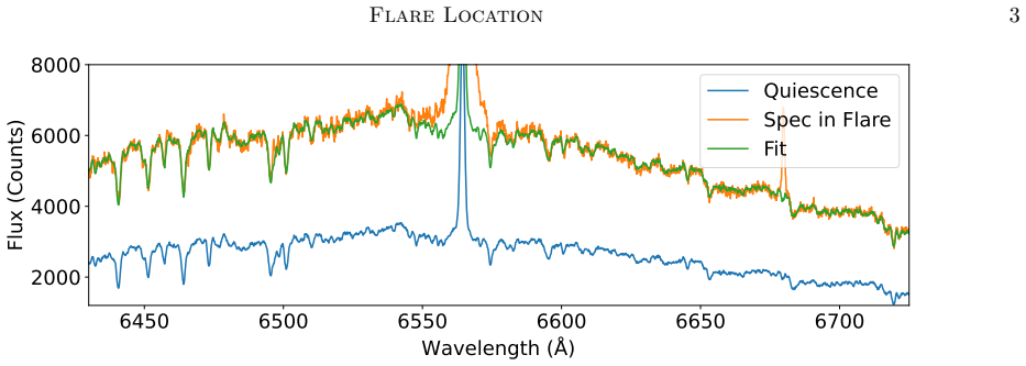


Figures from the paper (6 more)



Reference graph
Works this paper leans on
-
[1]
Abdel-Sattar, W., Mawad, R., & Moussas, X. 2018, Advances in Space Research, 62, 2701, doi: 10.1016/j.asr.2018.07.024 Abdurro’uf, Accetta, K., Aerts, C., et al. 2022, ApJS, 259, 35, doi: 10.3847/1538-4365/ac4414 Astropy Collaboration, Robitaille, T. P., Tollerud, E. J., et al. 2013, A&A, 558, A33, doi: 10.1051/0004-6361/201322068 Astropy Collaboration, Pr...
-
[2]
Bice, C. P., & Toomre, J. 2022, ApJ, 928, 51, doi: 10.3847/1538-4357/ac4be0
-
[3]
2024, A&A, 682, A176, doi: 10.1051/0004-6361/202347901
Bicz, K., Falewicz, R., & Pietras, M. 2024, A&A, 682, A176, doi: 10.1051/0004-6361/202347901
-
[4]
Caldwell, D. A., Tenenbaum, P., Twicken, J. D., et al. 2020, Research Notes of the American Astronomical Society, 4, 201, doi: 10.3847/2515-5172/abc9b3 Flare Location13 0.6 1.2 1.8 2.4 M 0.42 0.48 0.54 0.60 R 300 600 900 1200 Vesc 48 56 64 72 Ve 0.03650.03660.03670.0368 L 15 30 45 60 75 i 0.6 1.2 1.8 2.4 M 0.42 0.48 0.54 0.60 R 300 600 900 1200 Vesc 48 56...
arXiv 2020
-
[5]
2014, MNRAS, 444, 2525, doi: 10.1093/mnras/stu1605
Chen, Y., Girardi, L., Bressan, A., et al. 2014, MNRAS, 444, 2525, doi: 10.1093/mnras/stu1605
-
[6]
2019, A&A, 632, A105, doi: 10.1051/0004-6361/201936612
Chen, Y., Girardi, L., Fu, X., et al. 2019, A&A, 632, A105, doi: 10.1051/0004-6361/201936612
-
[7]
2000, A&A, 363, 1081
Claret, A. 2000, A&A, 363, 1081
2000
-
[8]
Davenport, J. R. A., Covey, K. R., Clarke, R. W., et al. 2019, ApJ, 871, 241, doi: 10.3847/1538-4357/aafb76
Show all 45 references
-
[9]
2016, The Journal of Open Source Software, 1, 24, doi: 10.21105/joss.00024
Foreman-Mackey, D. 2016, The Journal of Open Source Software, 1, 24, doi: 10.21105/joss.00024
2016 doi
-
[10]
W., Lang, D., & Goodman, J
Foreman-Mackey, D., Hogg, D. W., Lang, D., & Goodman, J. 2013, PASP, 125, 306, doi: 10.1086/670067
2013 doi
-
[11]
Schmitt, J. H. M. M. 2022, A&A, 664, A105, doi: 10.1051/0004-6361/202142573 Gaia Collaboration, Vallenari, A., Brown, A. G. A., et al. 2023, A&A, 674, A1, doi: 10.1051/0004-6361/202243940
2022 doi
-
[12]
Gershberg, R. E. 1972, Ap&SS, 19, 75, doi: 10.1007/BF00643168
1972 doi
-
[13]
Gray, D. F. 2005, The Observation and Analysis of Stellar Photospheres, doi: 10.1017/CBO9781316036570 G¨ unther, M. N., Zhan, Z., Seager, S., et al. 2020, AJ, 159, 60, doi: 10.3847/1538-3881/ab5d3a
2005 doi
-
[14]
R., Millman, K
Harris, C. R., Millman, K. J., van der Walt, S. J., et al. 2020, Nature, 585, 357, doi: 10.1038/s41586-020-2649-2
2020 doi
-
[15]
Hunter, J. D. 2007, Computing in Science & Engineering, 9, 90, doi: 10.1109/MCSE.2007.55
2007 doi
-
[16]
2013, A&A, 553, A6, doi: 10.1051/0004-6361/201219058
Husser, T.-O., Wende-von Berg, S., Dreizler, S., et al. 2013, A&A, 553, A6, doi: 10.1051/0004-6361/201219058
2013 doi
-
[17]
J., Poppenh¨ ager, K., et al
Ilin, E., Schmidt, S. J., Poppenh¨ ager, K., et al. 2021a, A&A, 645, A42, doi: 10.1051/0004-6361/202039198
-
[18]
J., et al
Ilin, E., Poppenhaeger, K., Schmidt, S. J., et al. 2021b, MNRAS, 507, 1723, doi: 10.1093/mnras/stab2159
-
[19]
M., Twicken, J
Jenkins, J. M., Twicken, J. D., McCauliff, S., et al. 2016, in Society of Photo-Optical Instrumentation Engineers (SPIE) Conference Series, Vol. 9913, Software and Cyberinfrastructure for Astronomy IV, ed. G. Chiozzi & J. C. Guzman, 99133E, doi: 10.1117/12.2233418
2016 doi
-
[20]
S., L¨ uftinger, T., & Kochukhov, O
Kay, C., Airapetian, V. S., L¨ uftinger, T., & Kochukhov, O. 2019, ApJL, 886, L37, doi: 10.3847/2041-8213/ab551f
2019 doi
-
[21]
2016, ApJ, 826, 195, doi: 10.3847/0004-637X/826/2/195 14Li et al
Kay, C., Opher, M., & Kornbleuth, M. 2016, ApJ, 826, 195, doi: 10.3847/0004-637X/826/2/195 14Li et al. 14.650 14.665 14.680 14.695 14.710Parallax (mas) 0.42300 0.42304 0.42308 0.42312Period (days) 24 30 36 42 48 Vesin i (km/s) 16 12 8 4 0 V (km/s) 70 75 80 85 0 (deg) 135 120 1...
2016
-
[22]
Lammer, H., Lichtenegger, H. I. M., Kulikov, Y. N., et al. 2007, Astrobiology, 7, 185, doi: 10.1089/ast.2006.0128
2007
-
[23]
2023, Research in Astronomy and Astrophysics, 23, 015016, doi: 10.1088/1674-4527/aca506
Li, G.-W., Wu, C., Zhou, G.-P., et al. 2023, Research in Astronomy and Astrophysics, 23, 015016, doi: 10.1088/1674-4527/aca506
2023 doi
-
[24]
2024, ApJ, 971, 114, doi: 10.3847/1538-4357/ad55e8 Lightkurve Collaboration, Cardoso, J
Li, G.-W., Wang, L., Yuan, H.-L., et al. 2024, ApJ, 971, 114, doi: 10.3847/1538-4357/ad55e8 Lightkurve Collaboration, Cardoso, J. V. d. M., Hedges, C., et al. 2018, Lightkurve: Kepler and TESS time series analysis in Python, Astrophysics Source Code Library, record ascl:1812.0...
2024 doi
- [25]
-
[26]
Lomb, N. R. 1976, Ap&SS, 39, 447, doi: 10.1007/BF00648343
1976 doi
-
[27]
2022, A&A, 663, A140, doi: 10.1051/0004-6361/202142909
Lu, H.-p., Tian, H., Zhang, L.-y., et al. 2022, A&A, 663, A140, doi: 10.1051/0004-6361/202142909
2022 doi
-
[28]
2015, Research in Astronomy and Astrophysics, 15, 1095, doi: 10.1088/1674-4527/15/8/002
Luo, A.-L., Zhao, Y.-H., Zhao, G., et al. 2015, Research in Astronomy and Astrophysics, 15, 1095, doi: 10.1088/1674-4527/15/8/002
2015 doi
- [29]
-
[30]
2022, ApJ, 935, 104, doi: 10.3847/1538-4357/ac77f9
Charbonneau, D. 2022, ApJ, 935, 104, doi: 10.3847/1538-4357/ac77f9
2022 doi
-
[31]
2023, MNRAS, 522, 4392, doi: 10.1093/mnras/stad1078
Menezes, F., Valio, A., Netto, Y., et al. 2023, MNRAS, 522, 4392, doi: 10.1093/mnras/stad1078
2023 doi
-
[32]
2003, A&A, 397, 147, doi: 10.1051/0004-6361:20021560
Ventura, P. 2003, A&A, 397, 147, doi: 10.1051/0004-6361:20021560
2003 doi
-
[33]
Reiners, A., Sch¨ ussler, M., & Passegger, V. M. 2014, ApJ, 794, 144, doi: 10.1088/0004-637X/794/2/144
2014 doi
-
[34]
Sasso, C., Andretta, V., Terranegra, L., & Gomez, M. T. 2017, A&A, 604, A50, doi: 10.1051/0004-6361/201730676
2017 doi
-
[35]
Scargle, J. D. 1982, ApJ, 263, 835, doi: 10.1086/160554
1982 doi
-
[36]
J., Kauristie, K., Aylward, A
Schrijver, C. J., Kauristie, K., Aylward, A. D., et al. 2015, Advances in Space Research, 55, 2745, doi: 10.1016/j.asr.2015.03.023
2015 doi
-
[37]
Schuessler, M., & Solanki, S. K. 1992, A&A, 264, L13
1992
-
[38]
Strassmeier, K. G. 2009, A&A Rv, 17, 251, doi: 10.1007/s00159-009-0020-6
2009 doi
-
[39]
W., Winn, J
Sullivan, P. W., Winn, J. N., Berta-Thompson, Z. K., et al. 2015, ApJ, 809, 77, doi: 10.1088/0004-637X/809/1/77
2015 doi
-
[40]
2019, Astrobiology, 19, 64, doi: 10.1089/ast.2017.1794
Davenport, J. 2019, Astrobiology, 19, 64, doi: 10.1089/ast.2017.1794
2019
-
[41]
M., Odert, P., Leitzinger, M., et al
Veronig, A. M., Odert, P., Leitzinger, M., et al. 2021, Nature Astronomy, 5, 697, doi: 10.1038/s41550-021-01345-9
2021 doi
-
[42]
E., et al
Virtanen, P., Gommers, R., Oliphant, T. E., et al. 2020, Nature Methods, 17, 261, doi: 10.1038/s41592-019-0686-2
2020 doi
-
[43]
J., Newton, E
Wright, N. J., Newton, E. R., Williams, P. K. G., Drake, J. J., & Yadav, R. K. 2018, MNRAS, 479, 2351, doi: 10.1093/mnras/sty1670
2018 doi
-
[44]
2019, ApJS, 241, 29, doi: 10.3847/1538-4365/ab0d28
Yang, H., & Liu, J. 2019, ApJS, 241, 29, doi: 10.3847/1538-4365/ab0d28
2019 doi
-
[45]
2025, A&A, 695, A21, doi: 10.1051/0004-6361/202453120
Yang, H., Cheng, X., Liu, J., et al. 2025, A&A, 695, A21, doi: 10.1051/0004-6361/202453120
2025 doi
Reviewed July 31, 2026 · model on record in the stance chip above.
Discussion (0). Sign in to comment.