REVIEW 4 major objections 3 minor 19 references
Efficient learning of bosonic unitaries beyond the Gaussian class
T0 review · 4 major / 3 minor · reviewed 2026-08-01 · deepseek-v4-flash
Pith's one-line read The paper tries to establish that the real obstacle to learning multimode bosonic unitaries is not non-Gaussianity by itself, but the irreducible mixing of non-Gaussian features with multimode entanglement. It claims that two broad non-Gaus
desk verdict A serious, novel paper whose main polynomial learning claims are conditional on a stated but unproved perturbative error-propagation assumption; deserves peer review, with the error-budget step as the focus. read the letter →
The pith
A machine-rendered reading of the paper's core claim, the machinery that carries it, and where it could break.
The reading
What carries the argument
The protocol rests on three structural tools. First, a multimode quantum Darmois–Skitovich theorem: under nontrivial passive (linear-optical) mixing, a product input can remain product only if all participating input states are Gaussian; this lets the learner identify the passive layers up to a limited gauge (permutations, local phase rotations, and mixing within covariance-degenerate Gaussian blocks). Second, an almost-sure activation theorem: for any non-Gaussian unitary, a random coherent probe produces a non-Gaussian output with probability one, so the exceptional coherent inputs that hide non-Gaussianity form a measure-zero set. Third, a self-calibrating single-mode unitary learner that
What would settle it
Compute, for a concrete non-Gaussian single-mode gate W embedded in a Gaussian-entanglable unitary with growing m, the exact output energy after the passive input layer under a fixed per-mode input energy; if the finite uniform intermediate evaluation-energy bound E** diverges with m, the polynomial query bound of Theorem 2 does not apply. Alternatively, construct a two-step instance where the perturbative error-propagation assumption underestimates the accumulated error by more than a constant factor—for example by numerically simulating the protocol with the estimated Gaussian counter-rotati
Extended reading notes
Core claim
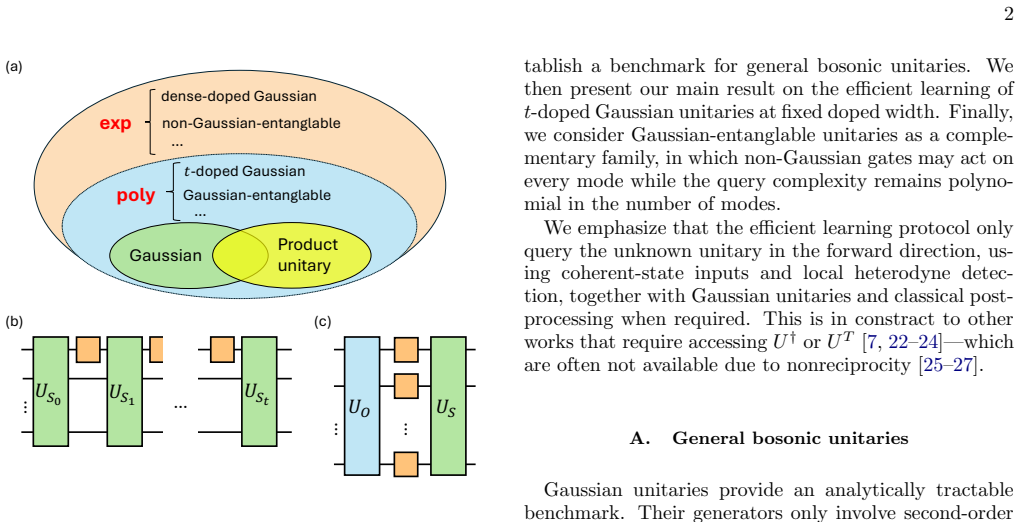
The paper's main results are two theorems. Theorem 1 shows that a t-doped Gaussian unitary U_doped = U_S (U_X ⊗ D) U_O, where the non-Gaussian block U_X acts on at most κt = O(1) modes, can be learned to error ε in energy-constrained diamond norm using M = poly(m) forward queries with coherent states and local heterodyne detection. Theorem 2 shows the same for Gaussian-entanglable unitaries U_ge = U_S (⊗_j W_j) U_O, where each W_j is an arbitrary single-mode unitary and the non-Gaussian layer can act on all m modes; the query complexity is poly(m, E*, 1/ε, log(1/δ)). Both protocols are forward-only, meaning they never require access to U† or U^T. The lower bound of Ω(E^{2m}) for general unit
Load-bearing premise
The polynomial query bounds assume that several energy quantities remain finite—the dynamical energy bound N_dyn, the output second-moment bound E_II, the per-probe output bound N_out, and the paper-specific finite uniform intermediate evaluation-energy bound E**—and that estimation errors from different steps add without cross-step amplification; if an intermediate energy blows up or errors amplify, the triangle-inequality composition no longer closes and the poly(m) claims
Editorial extensions
If this is right
- Structured photonic processors that interleave Gaussian operations with local nonlinear gates can be characterized with polynomially many forward queries, even when the number of modes is large.
- The exponential lower bound for general unitaries means the learnability boundary is set by the mixing of non-Gaussianity and entanglement, not by either resource alone.
- The quantum Darmois–Skitovich theorem gives a mode-resolved test for whether a passive linear-optical network genuinely mixes modes, which could be used as a diagnostic for hidden mixing.
- The activation theorem resolves probe selection: a random coherent probe is sufficient to reveal non-Gaussian dynamics, so adversarial hiding inputs are negligible.
- Learning from uncalibrated coherent probes removes the need for separate source calibration in coherent-state process tomography, up to an unavoidable phase-rotation gauge.
Reading between the lines
- Editorial inference: If the perturbative error-propagation assumption—that each step's error is computed assuming earlier steps are exact and errors add linearly—can be replaced by rigorous cross-step error bounds, the polynomial scaling would hold under weaker hypotheses; currently the triangle-inequality composition of errors in the proof relies on this assumption.
- Editorial inference: The Darmois–Skitovich theorem is exact; a finite-error version of it, as the paper itself notes, would extend the learning protocol to lossy or noisy settings where coherent outputs are only approximately product.
- Editorial inference: The lower bound Ω(E^{2m}) suggests that any efficient learner for a wider class of unitaries must exploit a promise that limits the number of modes on which non-Gaussian gates act jointly; families with blockwise non-Gaussian couplings of growing width are natural candidates for further study.
- Editorial inference: The uncalibrated-probe learner implies that calibration and process tomography can be merged; in practice this could reduce alignment requirements in photonic experiments, but the current protocol's complexity involves high powers of 1/ε, so numerical optimization of the constants would be a practical next step.
Editorial analysis
A structured set of objections, weighed in public.
Referee Report
Summary. The paper claims a tractability frontier for bosonic unitary learning. It proves a lower bound Ω(E^{2m}) for general m-mode unitaries under an energy constraint, and provides two positive results: t-doped Gaussian unitaries and Gaussian-entanglable unitaries can be learned with poly(m) queries using forward-only coherent-state probes, heterodyne detection, Gaussian operations, and classical post-processing. The proofs rely on a multimode quantum Darmois–Skitovich theorem, an almost-sure activation theorem for non-Gaussian unitaries, and a method for learning from uncalibrated coherent inputs. The main theorems are supported by extensive supplemental derivations and explicit sample-complexity expressions, but they are conditional on several additional energy-finiteness conditions and on an explicitly stated perturbative error-propagation assumption.
Significance. If fully established, the results are significant: they extend efficient bosonic process learning beyond the Gaussian class and identify the irreducible mixing of non-Gaussianity with multimode entanglement as the key complexity obstruction. The structural theorems—particularly the multimode Darmois–Skitovich theorem and the almost-sure activation theorem—are likely to be of independent interest beyond the learning application. The paper is also commendable for providing explicit protocols, explicit query-complexity bounds, and a detailed supplement. However, the central polynomial-query claims are not yet fully proven because the error-composition argument rests on an unproved perturbative approximation, and several energy conditions are assumed rather than derived from the stated physical constraints.
major comments (4)
- [Supplemental Note II A; Theorem S27, Eqs. (S459)–(S469)] The proof of the polynomial query bound uses an explicit 'perturbative error-propagation assumption' (Supplemental Note II A), under which each step's error is computed assuming previous steps are exact and total error is the sum. In Theorem S27, Eq. (S459) applies the triangle inequality, but the individual bounds (S460)–(S468) are only derived for exact intermediate channels. In particular, the third term (S466)–(S467) uses the uniform intermediate energy bound E** defined from the exact U_final in Eq. (S452), whereas the actual data for the local reconstruction W~'_j are obtained after approximate counter-rotations U~_S and U~_O2. No argument shows that Theorem S23 applies to those data with the same E**, nor that the local reconstruction error is Lipschitz in the preceding errors. Thus the composition (S469) is asserted, not derived. This is load-bearing for Theorems 1 and 2.
- [Theorems 1, 2 and Eq. (1)] The polynomial bounds are conditional on energy-finiteness conditions that are not implied by Eq. (1): N_dyn, E_II, and E**. In Theorem 2, E** is defined via Eq. (S452) from the exact U_final, which is unknown during the protocol; no verifiable condition is given. Theorem 1 similarly requires Proposition 10's N_dyn < ∞, a supremum over an unbounded set of states that is not guaranteed by bounded probe/output energies. The class of unitaries for which the protocols run in poly(m) is therefore not characterized by the stated physical assumptions, and no check is offered to certify these conditions.
- [Theorem 11, Eqs. (23)–(24)] The benchmark is presented as a tractability frontier, but the upper bound (24) relies on the unproved assumption 'Assume that the cutoff-L coherent-probe reconstruction is stable,' and the effective cutoff dimension d_L with L = max{K, 256 E_U(K)/ε²} can be much larger than the d_E used in the lower bound. Hence the upper bound is not a matching converse, and the frontier between the general lower bound and the two polynomial families is not quantitatively closed. The lower bound itself appears sound, but the 'frontier' claim should be calibrated.
- [Theorem S23 / Proposition 10] The single-mode uncalibrated learning theorem assumes N_dyn < ∞ for W_gf and N_out < ∞. These are used to set the cutoff R and to control the polar completion (Lemma S22). For many non-Gaussian unitaries the dynamical bound is finite, but for unitaries with unbounded energy growth N_dyn can be infinite. The theorems restrict to the finite case, which is an extra structural promise not visible in the main-text statement 'an arbitrary single-mode unitary.' The abstract and Section II overstate the reach of Theorem 9 if the finite-energy condition is not highlighted there.
minor comments (3)
- [Throughout] Typographical errors: 'Gaussian untiaries' (Section I.B), 'constract' (Section I), 'Gaussinity' (Supplemental Remark S16), 'exppoly' (Fig. 1 caption).
- [Theorem 11] The parameter C in Eq. (24) is not specified; an order bound with an unknown constant C≥5 makes the comparison with the lower bound loose. Please state the best available explicit value or explain why it is protocol-dependent.
- [Theorem S27 / Eq. (S452)] The quantity E** is defined in the supplement after Eq. (S452) but is cited in the main-text Theorem 2. Please define it in the main text or give a precise reference to the supplemental equation.
Circularity Check
No circularity: the unitary-learning theorems are new statements built on independent state-learning subroutines; the explicit perturbative error-propagation assumption is a proof gap, not a circular reduction.
full rationale
The derivation chain does not reduce any prediction to its inputs. Theorems 1 and 2 establish new process-learning statements—unitary learning, not just state learning—with forward-only protocols. The machinery inherited from the authors' own [16] (Gaussian disentangling, passive-separable shadow tomography, Gaussian-entanglable state tomography) is used as a state-learning subroutine and is external published evidence; it is load-bearing but not circular, because the unitary-level claims require new steps proved in the Supplement: the quantum Darmois–Skitovich rigidity (Theorem 5 / Proposition 6), the almost-sure activation theorems (Theorem 7 / Proposition 8), and uncalibrated-coherent-probe unitary reconstruction (Theorem 9 / Proposition 10). No equation is shown to equal another by construction, and no fitted parameter is renamed as a prediction. The finite-energy quantities N_dyn, E_II, and E** are stated assumptions rather than derived outputs, so they do not constitute circularity. The main flagged issue is Supplemental Note II A's explicit 'perturbative error-propagation assumption' and the four-term triangle-inequality accounting in Theorem S27, Eqs. (S449)–(S469): per-step bounds are proven assuming preceding steps are exact, and closing the telescoping sum for the actual approximate counter-rotations is asserted. This is a correctness/completeness gap, not an equivalence-by-definition or fitted-input circularity, so it does not raise the circularity score.
Assumptions & free parameters
assumptions (8)
- standard math Classical (vector) Skitovich–Darmois theorem: independent random vectors with two independent linear forms having nonsingular coefficient matrices must be Gaussian.
- standard math Holomorphic identity theorem and real-analytic zero-set theorem: a nonzero holomorphic/real-analytic function vanishes on a set of positive Lebesgue measure only if it vanishes identically.
- standard math Bargmann–Fock characterization of pure Gaussian states via the differential witness J_{ijk}[f] = 0 iff f is an exponential of a quadratic.
- domain assumption Finite dynamical energy for probed unitaries: output second moments ≤ mE_II, per-mode mean photon number of queried outputs ≤ N_out, and N_dyn := sup_{φ∈H≤J} ⟨φ|W† n̂ W|φ⟩ < ∞.
- ad hoc to paper Finite uniform intermediate evaluation-energy E** < ∞ bounding the energy entering every effective single-mode channel after the Gaussian/passive counter-rotations.
- ad hoc to paper Perturbative error-propagation assumption: per-step reconstruction errors are computed assuming all preceding steps are exact, and total error is taken as the sum.
- ad hoc to paper Stability of the cutoff-L coherent-probe algebraic reconstruction for general unitaries (conditioning/invertibility of the interpolation map).
- domain assumption Correctness and efficiency of the state-learning subroutines from Ref. [16] (Gaussian disentangling, passive-separable shadow tomography) and Ref. [8] (t-doped state compression, state tomography).
Cite this review
Pith. "Pith review of Efficient learning of bosonic unitaries beyond the Gaussian class." pith.science (2026). https://pith.science/paper/OH5SG3GQ
@misc{pith2026260727534,
  author       = {Pith},
  title        = {Pith review of: Efficient learning of bosonic unitaries beyond the Gaussian class},
  year         = {2026},
  howpublished = {\url{https://pith.science/paper/OH5SG3GQ}},
  note         = {Machine review of arXiv:2607.27534}
}
abstract
Multimode quantum processes are generally difficult to learn, due to the large dimensionality and complex entanglement structure beyond the Gaussian class. Here, we show that the fundamental obstruction is not non-Gaussianity itself, but the buildup of irreducible multimode non-Gaussian correlations. We establish a tractability frontier for bosonic unitary learning: a general $m$-mode unitary with input energy at most $E$ per mode requires at least $\Omega(E^{2m})$ channel uses, whereas two broad non-Gaussian families---$t$-doped Gaussian unitaries and Gaussian-entanglable unitaries---can be learned with resources polynomial in $m$. The latter can exhibit both extensive non-Gaussianity and strong multimode entanglement. Our forward-only protocols use coherent-state probes, Gaussian operations, local heterodyne detection, and classical post-processing to identify the global Gaussian mixing and reduce the remaining task to single- or few-mode learning. The analysis also yields a multimode quantum Darmois--Skitovich theorem showing that mode-spreading passive networks preserve product structure only for Gaussian input states, an almost-sure activation theorem for non-Gaussian processes showing that non-Gaussian unitaries yield non-Gaussian outputs for almost all coherent input states, and a method for learning unitaries from uncalibrated coherent probes. Our results identify that complexity of learning arises from irreducible mixing of non-Gaussianity and entanglement, rather than either resource alone.
Figures


Reference graph
Works this paper leans on
-
[1]
The centered amplitudes spanC x, the minimum distanced min := mini<j ∥βi−βj∥2 is positive, and the Bargmann phase unwrapping condition holds with marginζ >0
-
[2]
, βd are unisolvent for holomorphic polynomials of total degree at mostr
The pointsβ 1, . . . , βd are unisolvent for holomorphic polynomials of total degree at mostr
-
[3]
The coherent coefficient matrixC= h c(x) r (β1)· · ·c(x) r (βd) i is invertible, andκ C :=∥C −1∥∞
-
[4]
There exists Ndyn such thatN (x) Wg (q)≤N dyn, and the cutoffrsatisfiesr≥ l 256Ndyn ϵ2 m
LetG=D(γ)Γ(R)be the physical coherent gauge from Lemma S38, and defineW g :=W ⋆G†. There exists Ndyn such thatN (x) Wg (q)≤N dyn, and the cutoffrsatisfiesr≥ l 256Ndyn ϵ2 m . LetD ⋆ := maxi<j ∥βi −β j∥2. Let∆ dist,∆ H ,L (x) geom,η 0,L (x) C ,L ph,B x,L (x) QR, andρ (x) QR be the constants from the preceding lemmas. Chooseη stab >0such that ηstab ≤η 0,(S76...
-
[5]
The identified mode setχ coh provide output state with a trace distance error p ϵcoh/2
Learning of the remaining Gaussian unitary Recall that we proposed Steps (RE1’) and (RE2’) in Supplemental Note III D 1 to probe the unitaryU t,rest with coherent state|α (k)⟩and identify the modes that stably output coherent states. The identified mode setχ coh provide output state with a trace distance error p ϵcoh/2. In Steps (STU1’)-(STU8’) of Supplem...
-
[6]
Task LetU(ρ) :=U ρ U† be an arbitrary unknownm-mode unitary channel on the bosonic Hilbert spaceH. Without loss of generality, we evaluate the learning error in the energy-constrained diamond norm ∥V∥ mE ⋄ := sup Tr[( bHm⊗I)ρ]≤mE (V ⊗id)(ρ) 1, H m = mX s=1 a† sas + m 2 ,(S842) whereEis the per-mode physical input-energy upper bound. The learning task is n...
-
[7]
, αm)∈C m.(S848) Their total photon number is⟨α | bN|α ⟩=∥α∥ 2
Probe states and measurement We use multimode coherent probe states |α⟩ := mO s=1 |αs⟩,α= (α 1, . . . , αm)∈C m.(S848) Their total photon number is⟨α | bN|α ⟩=∥α∥ 2
-
[8]
On the output, we perform heterodyne detection with POVM Π(β) =π −m |β⟩⟨β|,β= (β 1,
Thus the corresponding physical energy is∥α∥ 2 2 + m 2 , and the probe respects the input-energy constraint whenever∥α∥ 2 2 ≤m E− 1 2 . On the output, we perform heterodyne detection with POVM Π(β) =π −m |β⟩⟨β|,β= (β 1, . . . , βm)∈C m.(S849) 102 Equivalently, a single shot produces the real vector y(ℓ) α = 2 Reβ (ℓ) α,1,2 Imβ (ℓ) α,1, . . . ,2 Reβ(ℓ) α,m...
Show all 19 references
-
[9]
Why multiple coherent probes are necessary A single probe state cannot determine an arbitraryD-dimensional unitary. Indeed, up to a global phase, the target unitary channel onH ≤L hasD 2 −1 real degrees of freedom, whereas the output generated by one fixed coherent probe is a ...
-
[10]
More explicitly, define Φ∈C M×D 2 ,Φ r,(n,n′) := α(r) n α(r) n′ √ n!n ′! ,n,n ′ ∈ JL.(S862) Here the column index (n,n ′) ranges overJ L × JL in any fixed order
Estimator of the process tensor by interpolation Fix a finite probe set AL = α(r) ∈C m M r=1, M≥D 2, D=|J L|= L+m m ,(S861) and assume that the associated interpolation matrix has full column rank. More explicitly, define Φ∈C M×D 2 ,Φ r,(n,n′) := α(r) n α(r) n′ √ n!n ′! ,n,n ′...
-
[11]
Reconstruction of the unitary matrix We now recover the matrix ofV L from the estimated process tensor. For eachn∈ J L, define then-th column vector ofV L by u(n) := (VL)jn j∈JL ∈C D.(S871) Then (S860) can be written compactly as Enn′ =u (n)u(n′)†,n,n ′ ∈ JL,(S872) whereE nn′ ...
-
[12]
We assume throughout that Φ has full column rank
Uniform estimation error for the sampled values Recall the probe set defined byA L ={α (r)}M r=1 ⊂C m, M≥D 2, D= L+m m , and the associated design matrix Φr,(n,n′) = α(r) n α(r) n′ √ n!n ′! ,forn,n ′ ∈ JL. We assume throughout that Φ has full column rank. For each probe index ...
-
[13]
Recall the vector form of the reconstruction problemg jk = Φe jk,and bejk = Φ†bgjk
Propagation through the interpolation map Let us fixj,k∈ J L. Recall the vector form of the reconstruction problemg jk = Φe jk,and bejk = Φ†bgjk. Hence, we have bejk −e jk = Φ†bgjk −g jk .(S886) To quantify the worst-case entrywise error, define the stability constant µ∞(Φ) :=...
-
[14]
(S890) immediately yields the shot requirement needed to achieve a target entrywise process-tensor accuracy
RMSE and total query complexity Eq. (S890) immediately yields the shot requirement needed to achieve a target entrywise process-tensor accuracy. Indeed, if one requires ∆ E ≤τwith probability at least 1−δ, it suffices to choose N≥C 2 rob µ∞(Φ)2 νmax τ −2 log M D2 δ .(S891) Sin...
-
[15]
Within the admissible energy range, successful reconstruction requires two conditions
Consequences for probe design The energy constraint restricts the admissible probe set toA L ⊆ α∈C m ∥α∥2 2 ≤N probe ,forN probe ≤ m(E−1/2). Within the admissible energy range, successful reconstruction requires two conditions. First, the interpolation matrix Φ must have full ...
-
[16]
Letq :=⌊m(E−1/2)⌋,and dE := dim(H ≤q) = q+m m
A rigorous lower bound from an energy-accessible code subspace The lower bound should depend on the dimension of a subspace that is genuinely accessible under the input- energy boundE, not on the truncation dimension chosen later for the upper bound. Letq :=⌊m(E−1/2)⌋,and dE :...
-
[17]
Proposition S50(Local stability of the reconstruction map).LetV L be a unitary onH ≤L withD= dim(H ≤L)
Stability of the algebraic reconstruction We next quantify how errors in the reconstructed process tensor propagate to the estimated finite-dimensional unitary. Proposition S50(Local stability of the reconstruction map).LetV L be a unitary onH ≤L withD= dim(H ≤L). Let Enn′ =u ...
-
[18]
ChooseLand a full-space unitary extensionVas in Theorem S49, but with accuracy parameterϵ model instead ofϵ
Upper bound from coherent probes, heterodyne data, and interpolation We now combine the effective-dimension reduction with the interpolation bound from Supplemental Note IV C and the reconstruction stability of Proposition S50. ChooseLand a full-space unitary extensionVas in T...
-
[19]
The lower bound is unconditional
A compact summary We now summarize the preceding analysis in a form that makes the lower and upper bounds directly comparable. The lower bound is unconditional. For the upper bound, we isolate the experimentally meaningful ingredients of the coherent-probe heterodyne protocol,...
Reviewed August 1, 2026 · model on record in the stance chip above.
Discussion (0). Continue with ORCID to comment.