When, why, and how do diffusion posterior samplers fail? A finite-sample lens
Pith reviewed 2026-06-29 08:07 UTC · model grok-4.3
The pith
Diffusion posterior samplers produce wrong distributions because they misestimate posterior spread at intermediate timesteps.
A machine-rendered reading of the paper's core claim, the machinery that carries it, and where it could break.
Core claim
Popular posterior sampling approximations in diffusion models tend to under- or over-estimate the spread of the posterior at intermediate timesteps. This misestimation arises solely from a multimodal prior combined with inaccurate spread at intermediate times and produces downstream errors such as sensitivity to early stopping time, inaccurate relative weighting of posterior modes, and hallucination of both prior modes absent from the posterior and likelihood modes unsupported by the prior.
What carries the argument
The finite-sample perspective on posterior sampling, which approximates the true posterior to arbitrary precision in the limit of infinite training set size for any forward model and prior.
If this is right
- Samplers exhibit sensitivity to the choice of early stopping time.
- Relative weighting between distinct posterior modes becomes inaccurate.
- Hallucinations appear both of prior modes absent from the posterior and of likelihood modes unsupported by the prior.
- The same errors arise from a multimodal prior alone without requiring a nonlinear measurement model or a multimodal posterior.
Where Pith is reading between the lines
- Correcting the spread estimate at intermediate steps could reduce hallucinations without changing the diffusion architecture.
- The diagnostic could be applied to test whether new likelihood approximations fix the spread error before they are deployed on real data.
- Similar finite-sample checks might expose analogous spread misestimation in other generative sampling procedures that rely on approximate likelihoods.
Load-bearing premise
The learned distribution approaches the true posterior arbitrarily closely once the training set grows large enough, regardless of the forward model or prior.
What would settle it
A controlled experiment in which popular diffusion samplers produce posterior samples whose spread at intermediate timesteps exactly matches the true posterior spread computed from infinite data would falsify the claimed source of the errors.
Figures
read the original abstract
Diffusion models have excellent capacity to model complex distributions of natural data, which has made them a popular and effective choice for posterior sampling in imaging inverse problems. Existing methods can incorporate any measurement model at inference time but must use an inexact approximation for the likelihood at intermediate timesteps for computational tractability. Although these approximations can often work well empirically, their downstream effect on the sampled posterior is poorly understood and can result in unexplained failures. To understand when, why, and how these likelihood approximations propagate to erroneous posterior distributions, we introduce a finite-sample perspective on posterior sampling that approximates the posterior to arbitrary precision as training set size tends towards infinity, for any forward model and prior distribution. Using this finite-sample lens, we observe that popular posterior sampling approximations tend to under- or over-estimate the spread of the posterior at intermediate timesteps, causing downstream consequences including sensitivity to early stopping time, inaccurate relative weighting of posterior modes, and hallucination, both of prior modes that are not in the posterior and likelihood modes that are not supported by the prior. Moreover, we find that the cause of these posterior errors requires neither a nonlinear measurement model nor a multimodal posterior, but can arise solely due to a multimodal prior and inaccurate posterior spread at intermediate sampling times. Our finite-sample posterior sampling approach is agnostic to the type of likelihood approximation and the type of (linear or nonlinear) forward model, and can thus serve as a drop-in diagnostic to evaluate the accuracy and failure modes of existing and future posterior samplers.
Editorial analysis
A structured set of objections, weighed in public.
Referee Report
Summary. The paper introduces a finite-sample perspective on diffusion posterior sampling for imaging inverse problems. This lens is claimed to approximate the true posterior to arbitrary precision in the infinite-training-set limit, for arbitrary forward models and priors. Using the lens, the authors report that standard inexact likelihood approximations at intermediate timesteps systematically misestimate posterior spread, producing downstream errors including early-stopping sensitivity, incorrect relative mode weights, and hallucinations of unsupported prior or likelihood modes. They further claim these errors arise from multimodal priors alone and that the diagnostic is agnostic to the choice of likelihood approximation or linearity of the measurement model.
Significance. If the finite-sample construction is rigorously justified and the reported observations hold under controlled experiments, the work supplies a practical diagnostic tool for a widely used class of posterior samplers. The isolation of spread misestimation as a sufficient cause (even for linear measurements and multimodal priors) is a concrete, testable insight that could guide the design of more accurate intermediate likelihood approximations.
major comments (2)
- [§3] §3 (finite-sample lens construction): the central claim that the approximation recovers the true posterior to arbitrary precision as training-set size tends to infinity, for any forward model and prior, is load-bearing for all subsequent observations. A formal statement and derivation (or reference to a convergence theorem) establishing this limit under the paper's assumptions on the data distribution and diffusion process is required; the current high-level description leaves open whether the construction remains valid when the forward model is nonlinear or the prior is multimodal.
- [§4.2–4.3] §4.2–4.3 (empirical observations of spread misestimation and hallucination): the reported failure modes are demonstrated via qualitative samples and a small number of quantitative metrics. To support the claim that spread misestimation is the root cause independent of nonlinearity, the experiments must include controlled ablations that isolate the effect of the likelihood approximation while holding the prior and measurement model fixed; without these controls, it is unclear whether the observed hallucinations are attributable to the finite-sample lens or to other implementation choices.
minor comments (2)
- [§3] Notation for the finite-sample posterior estimator is introduced without an explicit equation number; adding a numbered display equation would improve traceability when the lens is later used to diagnose specific samplers.
- [§4] Figure captions for the hallucination examples do not state the precise early-stopping timestep or the value of the likelihood approximation parameter used, making it difficult to reproduce the reported mode-weighting errors.
Simulated Author's Rebuttal
We thank the referee for the detailed and constructive report. The comments highlight important areas for strengthening the formal justification and experimental controls. We address each major comment below and commit to revisions that directly respond to the concerns raised.
read point-by-point responses
-
Referee: [§3] §3 (finite-sample lens construction): the central claim that the approximation recovers the true posterior to arbitrary precision as training-set size tends to infinity, for any forward model and prior, is load-bearing for all subsequent observations. A formal statement and derivation (or reference to a convergence theorem) establishing this limit under the paper's assumptions on the data distribution and diffusion process is required; the current high-level description leaves open whether the construction remains valid when the forward model is nonlinear or the prior is multimodal.
Authors: We agree that a formal statement is needed to make the convergence claim rigorous. In the revised manuscript we will add a dedicated subsection in §3 that states a proposition: under standard assumptions on the data distribution (compact support, Lipschitz score functions) and the diffusion process (variance-preserving schedule), the empirical measure induced by the finite training set converges in total variation to the true data measure as N→∞; the posterior sampler constructed from this empirical measure then converges to the true posterior for arbitrary (including nonlinear) forward models and multimodal priors. A proof sketch will be included, relying on consistency of kernel density estimates for the score and the continuous mapping theorem for the reverse SDE. This will explicitly cover the multimodal and nonlinear cases. revision: yes
-
Referee: [§4.2–4.3] §4.2–4.3 (empirical observations of spread misestimation and hallucination): the reported failure modes are demonstrated via qualitative samples and a small number of quantitative metrics. To support the claim that spread misestimation is the root cause independent of nonlinearity, the experiments must include controlled ablations that isolate the effect of the likelihood approximation while holding the prior and measurement model fixed; without these controls, it is unclear whether the observed hallucinations are attributable to the finite-sample lens or to other implementation choices.
Authors: We accept that stronger isolation is required. In the revision we will expand §4.2–4.3 with new controlled ablations on linear measurement models (e.g., Gaussian blur and downsampling) using a fixed multimodal prior (mixture of Gaussians in latent space). We will vary only the intermediate likelihood approximation (standard vs. our finite-sample correction) while keeping the diffusion model, sampler, and measurement operator identical, and report quantitative metrics including posterior variance at selected timesteps, mode-weighting error (KL between recovered and true mode probabilities), and hallucination rate (fraction of samples outside the true posterior support). These results will be presented alongside the existing qualitative examples. revision: yes
Circularity Check
No significant circularity identified
full rationale
The paper introduces a finite-sample perspective as a theoretical construction that recovers the true posterior in the N→∞ limit for arbitrary forward models and priors. This lens is used to diagnose consequences of existing likelihood approximations at intermediate timesteps. No equations or claims reduce by construction to fitted parameters, self-definitions, or load-bearing self-citations; the central diagnostic remains independent of the failure modes it identifies. The derivation chain is self-contained against external benchmarks.
Axiom & Free-Parameter Ledger
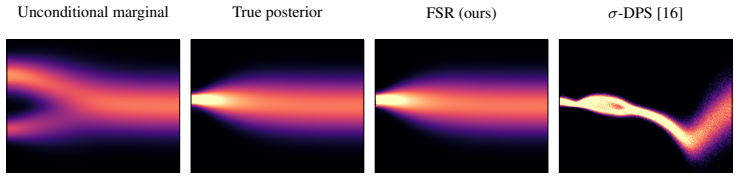
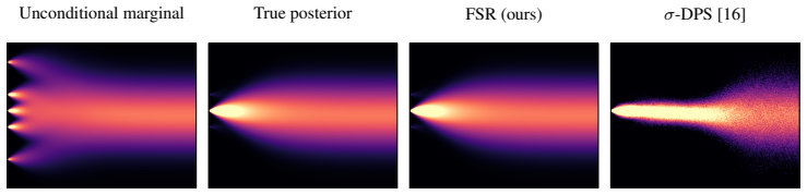
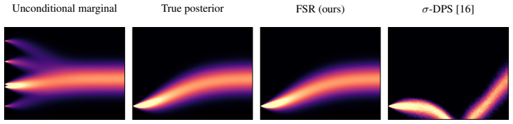
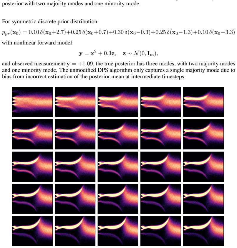
axioms (1)
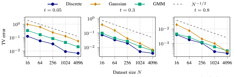
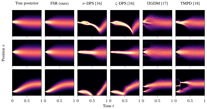
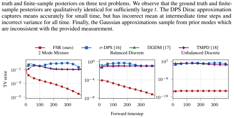
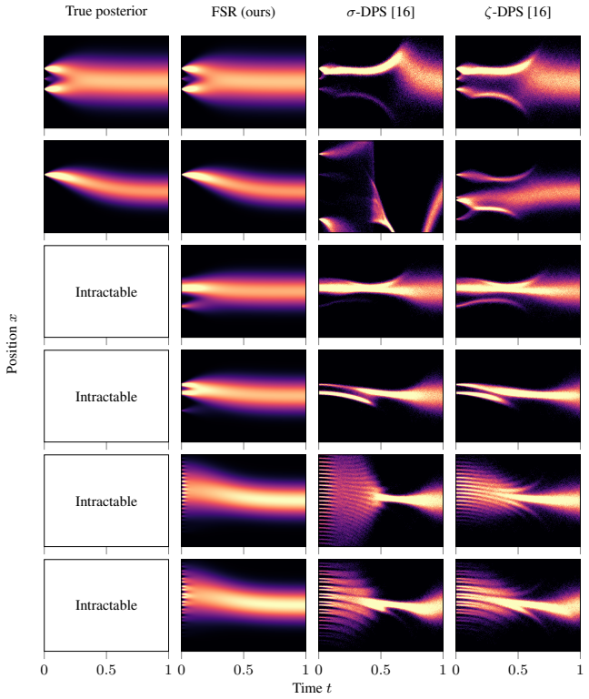
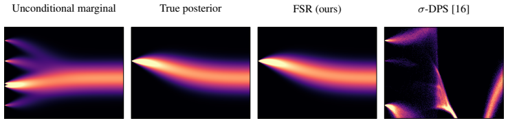
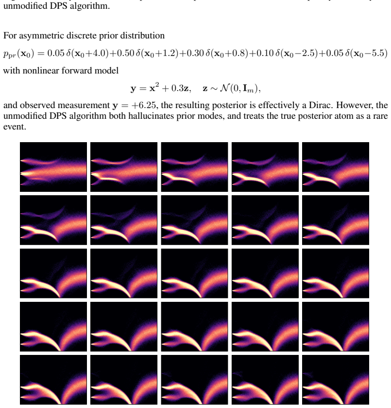
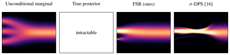
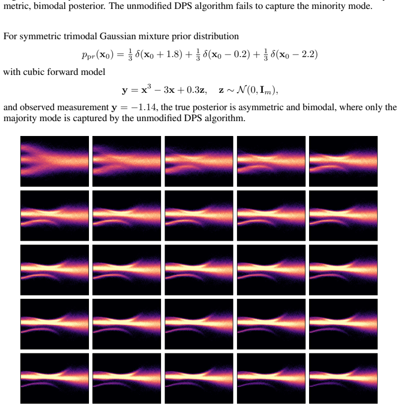
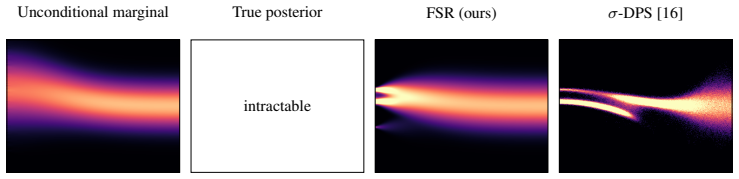
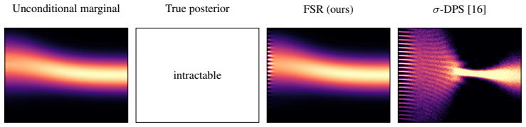
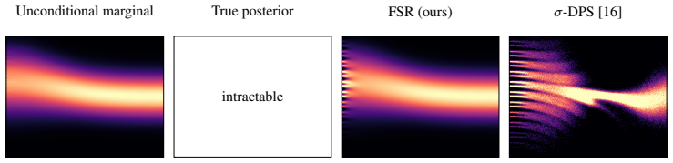
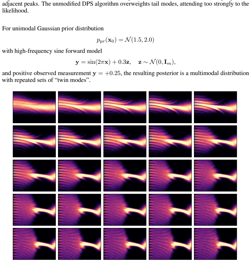
- domain assumption The posterior can be approximated to arbitrary precision as training set size tends towards infinity, for any forward model and prior distribution.
Reference graph
Works this paper leans on
-
[1]
Cambridge University Press, 2021
Ben Adcock and Anders C Hansen.Compressive Imaging: Structure, Sampling, Learning. Cambridge University Press, 2021
2021
-
[2]
Sullivan.Introduction to Uncertainty Quantification, volume 63 ofTexts in Applied Mathematics
T.J. Sullivan.Introduction to Uncertainty Quantification, volume 63 ofTexts in Applied Mathematics. Springer International Publishing, Cham, 2015. ISBN 978-3-319-23394-9 978-3-319-23395-6. doi: 10.1007/978-3-319-23395-6
-
[3]
Roger Ghanem, David Higdon, and Houman Owhadi, editors.Handbook of Uncertainty Quantification. Springer, Cham, 2017. ISBN 978-3-319-12384-4. doi: 10.1007/978-3-319-12385-1
-
[4]
Tomographic sparse view selection using the view covariance loss.IEEE Transactions on Pattern Analysis and Machine Intelligence, 2025
Jingsong Lin, Amirkoushyar Ziabari, Singanallur V Venkatakrishnan, Obaidullah Rahman, Gregery T Buzzard, and Charles A Bouman. Tomographic sparse view selection using the view covariance loss.IEEE Transactions on Pattern Analysis and Machine Intelligence, 2025
2025
-
[5]
PSC: Posterior sampling-based compression.Transactions on Machine Learning Research, 2025
Noam Elata, Tomer Michaeli, and Michael Elad. PSC: Posterior sampling-based compression.Transactions on Machine Learning Research, 2025. 13
2025
-
[6]
Bayes’ Rays: Uncertainty quantification in neural radiance fields.IEEE/CVF Conference on Computer Vision and Pattern Recognition (CVPR), 2024
Lily Goli, Cody Reading, Silvia Sellán, Alec Jacobson, and Andrea Tagliasacchi. Bayes’ Rays: Uncertainty quantification in neural radiance fields.IEEE/CVF Conference on Computer Vision and Pattern Recognition (CVPR), 2024
2024
-
[7]
Tyrrell Rockafellar and Stanislav Uryasev
R. Tyrrell Rockafellar and Stanislav Uryasev. Optimization of conditional value-at-risk.Journal of Risk, 2 (3):21–41, 2000. doi: 10.21314/JOR.2000.038
-
[8]
How should a robot assess risk? Towards an axiomatic theory of risk in robotics
Anirudha Majumdar and Marco Pavone. How should a robot assess risk? Towards an axiomatic theory of risk in robotics. InInternational Symposium on Robotics Research (ISRR), Puerto Varas, Chile, 2017
2017
-
[9]
Deep unsupervised learning using nonequilibrium thermodynamics
Jascha Sohl-Dickstein, Eric Weiss, Niru Maheswaranathan, and Surya Ganguli. Deep unsupervised learning using nonequilibrium thermodynamics. In Francis Bach and David Blei, editors,Proceedings of the 32nd International Conference on Machine Learning, volume 37 ofProceedings of Machine Learning Research, pages 2256–2265, Lille, France, July 2015. PMLR
2015
-
[10]
Denoising diffusion probabilistic models
Jonathan Ho, Ajay Jain, and Pieter Abbeel. Denoising diffusion probabilistic models. In H. Larochelle, M. Ranzato, R. Hadsell, M.F. Balcan, and H. Lin, editors,Advances in Neural Information Processing Systems, volume 33, pages 6840–6851. Curran Associates, Inc., 2020
2020
-
[11]
Kingma, Abhishek Kumar, Stefano Ermon, and Ben Poole
Yang Song, Jascha Sohl-Dickstein, Diederik P. Kingma, Abhishek Kumar, Stefano Ermon, and Ben Poole. Score-Based Generative Modeling through Stochastic Differential Equations. InInternational Conference on Learning Representations, October 2020
2020
-
[12]
Oxford University Press, 2025
Reinhard Heckel.Deep Learning for Computational Imaging. Oxford University Press, 2025
2025
-
[13]
InverseBench: Benchmarking plug-and-play diffusion priors for inverse problems in physical sciences
Hongkai Zheng, Wenda Chu, Bingliang Zhang, Zihui Wu, Austin Wang, Berthy Feng, Caifeng Zou, Yu Sun, Nikola Borislavov Kovachki, Zachary E Ross, Katherine Bouman, and Yisong Yue. InverseBench: Benchmarking plug-and-play diffusion priors for inverse problems in physical sciences. InThe Thirteenth International Conference on Learning Representations, 2025
2025
-
[14]
Agnimitra Dasgupta, Alexsander Marciano Da Cunha, Ali Fardisi, Mehrnegar Aminy, Brianna Binder, Bryan Shaddy, and Assad A. Oberai. Unifying and extending diffusion models through PDEs for solving inverse problems.Computer Methods in Applied Mechanics and Engineering, 448:118431, January 2026. doi: 10.1016/j.cma.2025.118431
-
[15]
An empirical Bayes approach to statistics
Herbert Robbins. An empirical Bayes approach to statistics. InProceedings of the Third Berkeley Symposium on Mathematical Statistics and Probability, 1954–1955, Volume I, pages 157–163, Berkeley and Los Angeles, 1956. University of California Press
1954
-
[16]
Diffusion posterior sampling for general noisy inverse problems
Hyungjin Chung, Jeongsol Kim, Michael Thompson Mccann, Marc Louis Klasky, and Jong Chul Ye. Diffusion posterior sampling for general noisy inverse problems. InThe Eleventh International Conference on Learning Representations, 2023
2023
-
[17]
Pseudoinverse-guided diffusion models for inverse problems
Jiaming Song, Arash Vahdat, Morteza Mardani, and Jan Kautz. Pseudoinverse-guided diffusion models for inverse problems. InInternational Conference on Learning Representations, 2023
2023
-
[18]
Tweedie Moment Projected Diffusions for Inverse Problems.Transactions on Machine Learning Research, July 2024
Benjamin Boys, Mark Girolami, Jakiw Pidstrigach, Sebastian Reich, Alan Mosca, and Omer Deniz Akyildiz. Tweedie Moment Projected Diffusions for Inverse Problems.Transactions on Machine Learning Research, July 2024
2024
-
[19]
Provably Robust Score-Based Diffusion Posterior Sampling for Plug-and-Play Image Reconstruction
Xingyu Xu and Yuejie Chi. Provably Robust Score-Based Diffusion Posterior Sampling for Plug-and-Play Image Reconstruction. InThe Thirty-eighth Annual Conference on Neural Information Processing Systems, November 2024
2024
-
[20]
Evan Scope Crafts and Umberto Villa. Benchmarking Diffusion Annealing-Based Bayesian Inverse Problem Solvers.IEEE Open Journal of Signal Processing, 6:975–991, 2025. doi: 10.1109/OJSP.2025. 3597867
-
[21]
Improving diffusion inverse problem solving with decoupled noise annealing
Bingliang Zhang, Wenda Chu, Julius Berner, Chenlin Meng, Anima Anandkumar, and Yang Song. Improving diffusion inverse problem solving with decoupled noise annealing. InProceedings of the IEEE/CVF Conference on Computer Vision and Pattern Recognition (CVPR), pages 20895–20905, June 2025
2025
-
[22]
Rethinking diffusion posterior sampling: From conditional score estimator to maximizing a posterior
Tongda Xu, Xiyan Cai, Xinjie Zhang, Xingtong Ge, Dailan He, Ming Sun, Jingjing Liu, Ya-Qin Zhang, Jian Li, and Yan Wang. Rethinking diffusion posterior sampling: From conditional score estimator to maximizing a posterior. InThe Thirteenth International Conference on Learning Representations, 2025
2025
-
[23]
Closed-form diffusion models
Christopher Scarvelis, Haitz Sáez de Ocáriz Borde, and Justin Solomon. Closed-form diffusion models. Transactions on Machine Learning Research, 2025. 14
2025
-
[25]
IEnSF: Iterative Ensemble Score Filter for Reducing Error in Posterior Score Estimation in Nonlinear Data Assimilation, October 2025
Zezhong Zhang, Feng Bao, and Guannan Zhang. IEnSF: Iterative Ensemble Score Filter for Reducing Error in Posterior Score Estimation in Nonlinear Data Assimilation, October 2025
2025
-
[26]
Score-based generative models are provably robust: An uncertainty quantification perspective
Nikiforos Mimikos-Stamatopoulos, Benjamin Zhang, and Markos Katsoulakis. Score-based generative models are provably robust: An uncertainty quantification perspective. InThe Thirty-Eighth Annual Conference on Neural Information Processing Systems, 2024
2024
-
[27]
Nishimura.Principles of magnetic resonance imaging
Dwight G. Nishimura.Principles of magnetic resonance imaging. Stanford University, 2010
2010
-
[28]
CRC Press, 2023
Xiangyang Tang.Spectral Multi-detector Computed Tomography (sMDCT): Data Acquisition, Image Formation, Quality Assessment and Contrast Enhancement. CRC Press, 2023
2023
-
[29]
Gradient descent provably solves nonlinear tomographic reconstruction.IEEE Transactions on Information Theory, 2026
Sara Fridovich-Keil, Fabrizio Valdivia, Gordon Wetzstein, Benjamin Recht, and Mahdi Soltanolkotabi. Gradient descent provably solves nonlinear tomographic reconstruction.IEEE Transactions on Information Theory, 2026
2026
-
[30]
G. E. Uhlenbeck and L. S. Ornstein. On the Theory of the Brownian Motion.Physical Review, 36(5): 823–841, September 1930. doi: 10.1103/PhysRev.36.823
-
[31]
Brian D. O. Anderson. Reverse-time diffusion equation models.Stochastic Processes and their Applications, 12(3):313–326, May 1982. doi: 10.1016/0304-4149(82)90051-5
-
[32]
Variational inference with normalizing flows
Danilo Rezende and Shakir Mohamed. Variational inference with normalizing flows. In Francis Bach and David Blei, editors,Proceedings of the 32nd International Conference on Machine Learning, volume 37 of Proceedings of Machine Learning Research, pages 1530–1538, Lille, France, July 2015. PMLR
2015
-
[33]
Estimation of non-normalized statistical models by score matching.Journal of Machine Learning Research, 6(24):695–709, 2005
Aapo Hyvärinen. Estimation of non-normalized statistical models by score matching.Journal of Machine Learning Research, 6(24):695–709, 2005
2005
-
[34]
A connection between score matching and denoising autoencoders
Pascal Vincent. A connection between score matching and denoising autoencoders.Neural Computation, 23(7):1661–1674, July 2011. doi: 10.1162/NECO_a_00142
-
[35]
Learning diffusion priors from observations by expectation maximization
François Rozet, Gérôme Andry, Francois Lanusse, and Gilles Louppe. Learning diffusion priors from observations by expectation maximization. InThe Thirty-Eighth Annual Conference on Neural Information Processing Systems, 2024
2024
-
[36]
Guided diffusion sampling on function spaces with applications to PDEs
Jiachen Yao, Abbas Mammadov, Julius Berner, Gavin Kerrigan, Jong Chul Ye, Kamyar Azizzadenesheli, and Anima Anandkumar. Guided diffusion sampling on function spaces with applications to PDEs. InThe Thirty-Ninth Annual Conference on Neural Information Processing Systems, 2026
2026
-
[37]
Sifan Wang, Zehao Dou, Siming Shan, Tong-Rui Liu, and Lu Lu. FunDiff: Diffusion models over function spaces for physics-informed generative modeling.Nature Communications, April 2026. doi: 10.1038/s41467-026-72292-0
-
[38]
KLIP: Localized distribution shift detection via KL-divergence with diffusion priors in inverse problems
Alireza Kheirandish, Jihoon Hong, and Sara Fridovich-Keil. KLIP: Localized distribution shift detection via KL-divergence with diffusion priors in inverse problems. InIEEE/CVF Conference on Computer Vision and Pattern Recognition (CVPR), 2026
2026
-
[39]
Conditional Image Generation with Score-Based Diffusion Models, November 2021
Georgios Batzolis, Jan Stanczuk, Carola-Bibiane Schönlieb, and Christian Etmann. Conditional Image Generation with Score-Based Diffusion Models, November 2021
2021
-
[40]
Diffusion models beat GANs on image synthesis
Prafulla Dhariwal and Alexander Quinn Nichol. Diffusion models beat GANs on image synthesis. In A. Beygelzimer, Y . Dauphin, P. Liang, and J. Wortman Vaughan, editors,Advances in Neural Information Processing Systems, 2021
2021
-
[41]
Elucidating the design space of diffusion-based generative models
Tero Karras, Miika Aittala, Samuli Laine, and Timo Aila. Elucidating the design space of diffusion-based generative models. InProceedings of the 36th International Conference on Neural Information Processing Systems, Nips ’22, Red Hook, NY , USA, 2022. Curran Associates Inc. ISBN 978-1-7138-7108-8
2022
-
[42]
DEFT: Efficient fine-tuning of diffusion models by learning the generalised $h$-transform
Alexander Denker, Francisco Vargas, Shreyas Padhy, Kieran Didi, Simon V Mathis, Riccardo Barbano, Vincent Dutordoir, Emile Mathieu, Urszula Julia Komorowska, and Pietro Lio. DEFT: Efficient fine-tuning of diffusion models by learning the generalised $h$-transform. InThe Thirty-Eighth Annual Conference on Neural Information Processing Systems, 2024
2024
-
[43]
Principled probabilistic imaging using diffusion models as plug-and-play priors
Zihui Wu, Yu Sun, Yifan Chen, Bingliang Zhang, Yisong Yue, and Katherine Bouman. Principled probabilistic imaging using diffusion models as plug-and-play priors. InThe Thirty-Eighth Annual Conference on Neural Information Processing Systems, 2024. 15
2024
-
[44]
Boffi, and Eric Vanden-Eijnden
Michael Albergo, Nicholas M. Boffi, and Eric Vanden-Eijnden. Stochastic interpolants: A unifying framework for flows and diffusions.Journal of Machine Learning Research, 26(209):1–80, 2025
2025
-
[45]
Albergo, Mark Goldstein, Nicholas M
Michael S. Albergo, Mark Goldstein, Nicholas M. Boffi, Rajesh Ranganath, and Eric Vanden-Eijnden. Stochastic interpolants with data-dependent couplings, September 2024
2024
-
[46]
Yaron Lipman, Ricky T. Q. Chen, Heli Ben-Hamu, Maximilian Nickel, and Matthew Le. Flow matching for generative modeling. InThe Eleventh International Conference on Learning Representations, 2023
2023
-
[47]
FlowDPS : Flow-driven posterior sampling for inverse problems
Jeongsol Kim, Bryan Sangwoo Kim, and Jong Chul Ye. FlowDPS : Flow-driven posterior sampling for inverse problems. InProceedings of the IEEE/CVF International Conference on Computer Vision (ICCV), pages 12328–12337, October 2025
2025
-
[48]
Exact Conditional Score-Guided Generative Modeling for Amortized Inference in Uncertainty Quantification, June 2025
Zezhong Zhang, Caroline Tatsuoka, Dongbin Xiu, and Guannan Zhang. Exact Conditional Score-Guided Generative Modeling for Amortized Inference in Uncertainty Quantification, June 2025
2025
-
[49]
Error estimates of a training-free diffusion model for high-dimensional sampling, January 2026
Pengjun Wang, Zezhong Zhang, Minglei Yang, Feng Bao, Yanzhao Cao, and Guannan Zhang. Error estimates of a training-free diffusion model for high-dimensional sampling, January 2026. 16 Contents A Related work 17 A.1 Generative posterior samplers . . . . . . . . . . . . . . . . . . . . . . . . . . . . 17 A.2 Benchmarking vs. understanding . . . . . . . . . ...
2026
-
[50]
the true posterior (where available), derived in Appendix D.1,
-
[51]
FSR: the finite-sample regime introduced in Section 4, 3.σ-DPS [16], defined in Equation (16) with unmodified prefactorσ −2 y , 4.ζ-DPS [16], defined in Equation (25) with modified prefactorζ/∥y− A(m 0|t(xt))∥2, 5.ΠGDM [17], defined in Equation (21), and
-
[52]
tail-event
TMPD [18], defined in Equation (22). The FSR and DPS methods are present for all problems, whileΠGDM and TMPD are only applicable when the measurement model is affine. Heatmaps use power-law normalization with exponent γ= 0.55 . The color ceiling is set per row to the 99th percentile of that row’s analytic field with flipping at the99.9th percentile to pr...
2000
discussion (0)
Sign in with ORCID, Apple, or X to comment. Anyone can read and Pith papers without signing in.