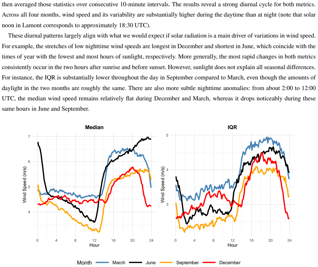
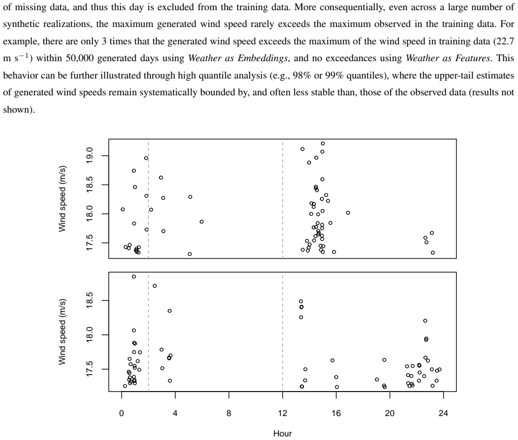
Stochastic weather generators for high-frequency wind vector time series
Pith reviewed 2026-06-27 14:58 UTC · model grok-4.3
The pith
Machine learning models using vector-quantized autoencoders generate minute-scale wind vector time series that capture diurnal volatility changes but fail to match extreme wind speed distributions.
A machine-rendered reading of the paper's core claim, the machinery that carries it, and where it could break.
Core claim
This work develops a range of machine learning models for generating realistic time series of surface wind vectors at a site in Lamont, Oklahoma based on more than 30 years of high quality measurements at the minute time scale. The data show complex diurnal structures in both wind speed and direction that would be challenging to capture with standard time series models, so we consider a number of machine learning approaches to producing a stochastic wind generator based on time vector-quantized variational autoencoders. We consider generating a day's worth of data at a time and generating a day of wind vectors conditional on the previous day's winds. We also study methods for incorporating a
What carries the argument
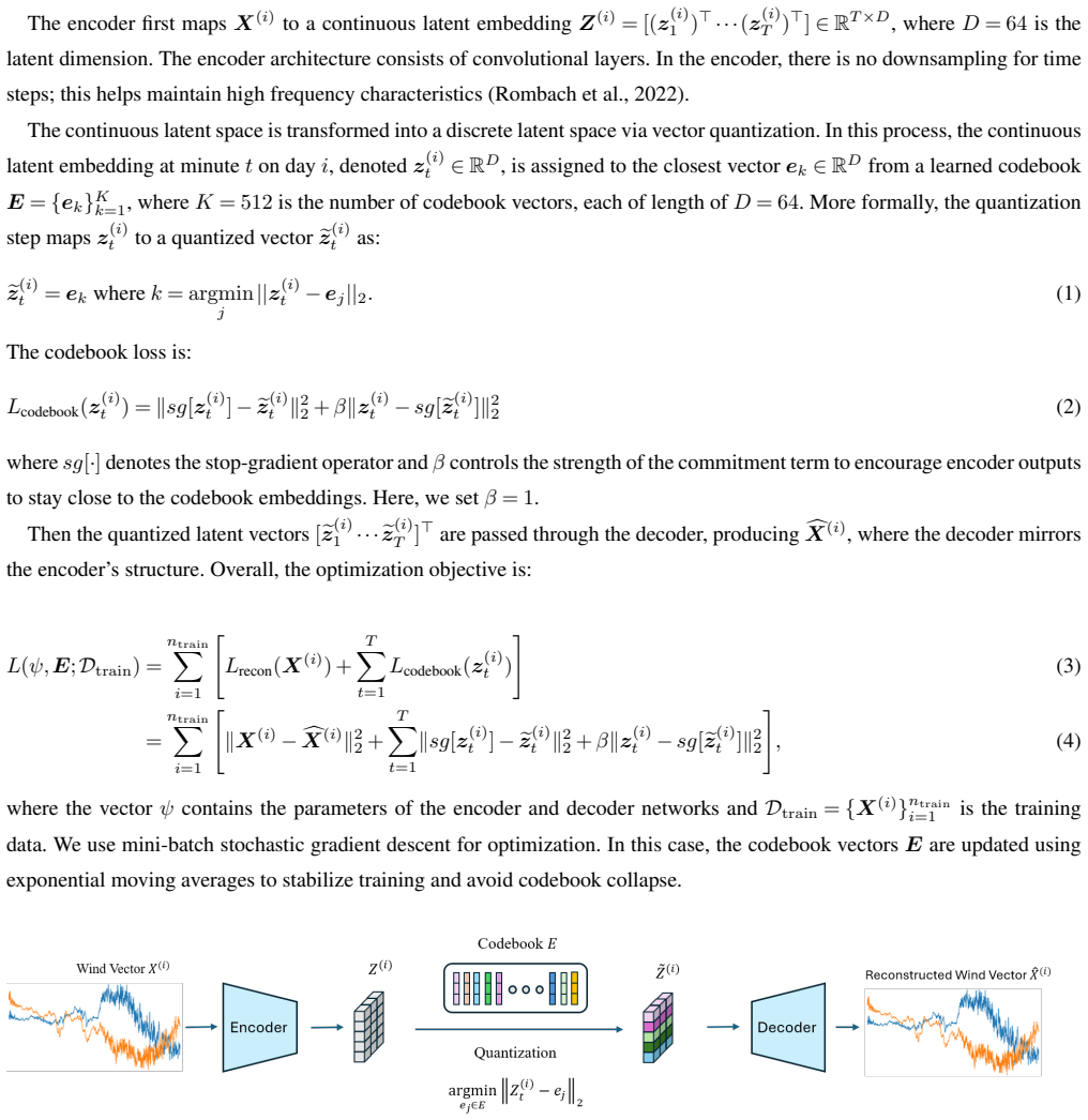
Time vector-quantized variational autoencoders (VQ-VAE) that generate daily wind vector sequences, either unconditionally or conditioned on the previous day's winds and optional discrete weather states.
If this is right
- The generators can supply minute-scale wind inputs to downstream models in wind energy, wildfire spread, and aviation.
- Diurnal volatility patterns in wind speed and direction are reproduced accurately enough for many applications.
- Extreme wind speed tails remain mismatched, limiting use in risk-sensitive settings.
- Incorporating weather state variables improves some features but does not resolve the extreme-value shortfall.
Where Pith is reading between the lines
- The same VQ-VAE conditioning approach could be tested on data from other months or sites to check whether the diurnal capture generalizes beyond the June restriction.
- Better extreme-value modeling might require hybrid methods that combine the current generators with separate tail models.
- If the diurnal volatility match holds, these generators could reduce reliance on parametric assumptions in high-frequency wind simulations for operational forecasting.
Load-bearing premise
That restricting analysis to a single site and the month of June, combined with the VQ-VAE architecture and chosen conditioning schemes, is sufficient to capture the full range of complex diurnal structures present in the minute-scale observations.
What would settle it
Compare the distribution of generated extreme wind speeds against held-out minute-scale observations from the same site in June; a clear mismatch in the upper tail would falsify the claim that the generators reproduce observed extremes.
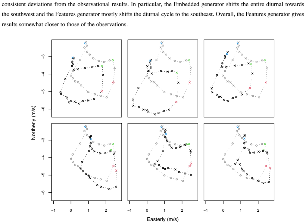
Figures
read the original abstract
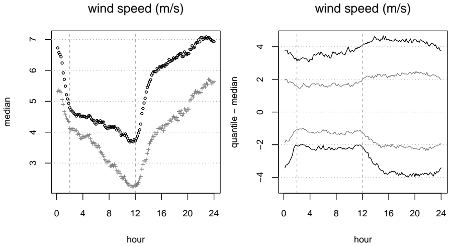
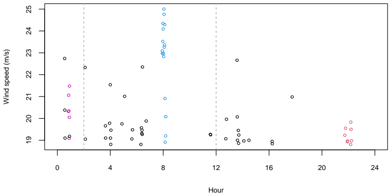
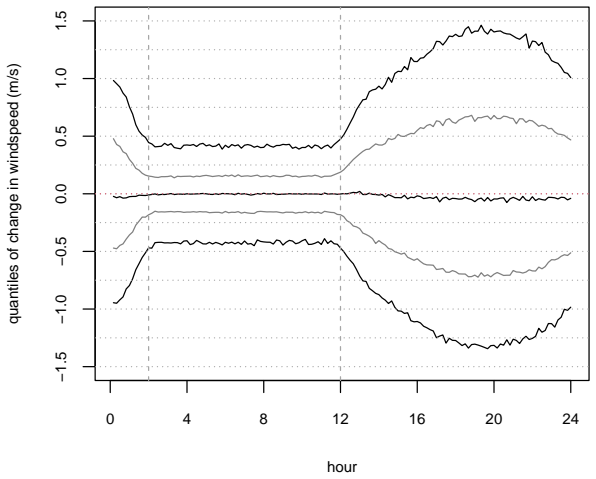
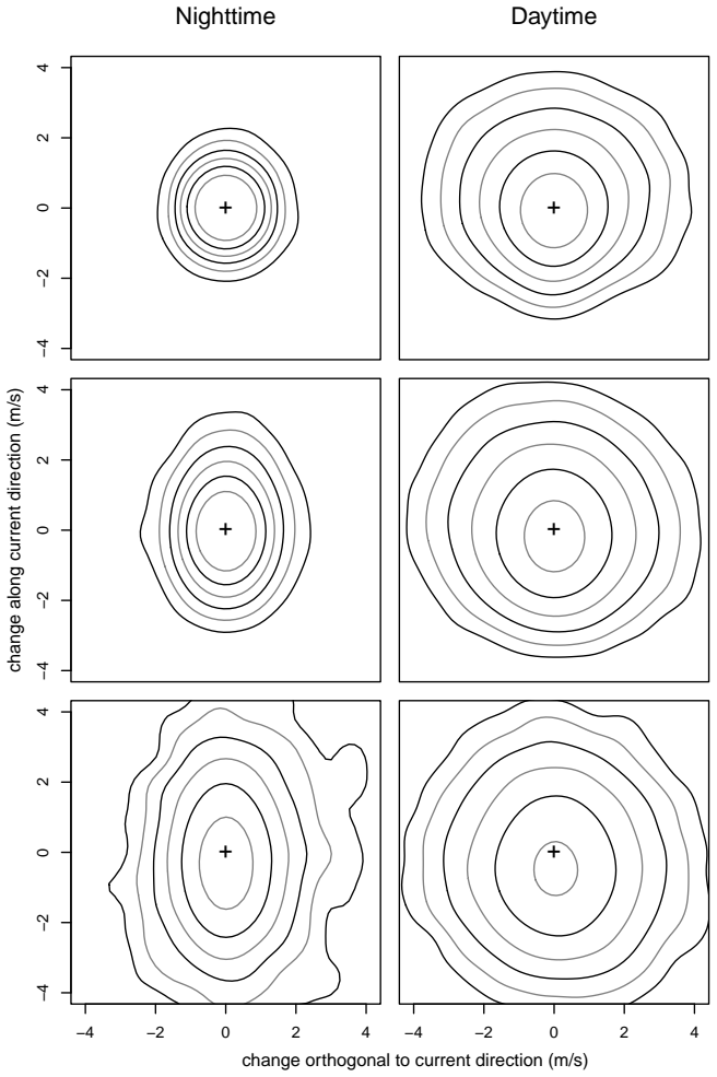
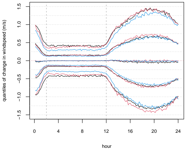
Surface winds can vary substantially from one minute to the next, so there is scope for studying its variation on this fine time scale. Restricting to the month of June to minimize seasonality, this work develops a range of machine learning models for generating realistic time series of surface wind vectors at a site in Lamont, Oklahoma based on more than 30 years of high quality measurements at the minute time scale. Such a generator could be used as an input into models from a range of disciplines, notably for wind energy, but also wildfire spread and aviation, among others. The data show complex diurnal structures in both wind speed and direction that would be challenging to capture with standard time series models, so we consider a number of machine learning approaches to producing a stochastic wind generator based on time vector-quantized variational autoencoders. We consider generating a day's worth of data at a time and generating a day of wind vectors conditional on the previous day's winds. We also study methods for incorporating a discrete weather state variable in the generator. We evaluate the generators using a wide range of formal and informal methods. The best of these generators can capture many but not all of the complex features present in the observational data. In particular, the best of our approaches accurately mimic diurnal changes in wind volatility but struggle to match the observed distribution of extreme wind speeds.
Editorial analysis
A structured set of objections, weighed in public.
Referee Report
Summary. The manuscript develops several VQ-VAE-based stochastic generators for minute-scale wind vector time series, restricted to June observations at a single Oklahoma site. It examines unconditional day-long generation, generation conditional on the prior day, and variants that incorporate a discrete weather state variable. Using a mix of formal and informal diagnostics, the authors conclude that the strongest models reproduce observed diurnal volatility patterns but do not reproduce the distribution of extreme wind speeds.
Significance. If the empirical findings are substantiated, the work supplies a practical exploratory template for high-frequency wind simulation that can accommodate complex diurnal structure, relevant to wind-energy, wildfire, and aviation applications. The explicit qualification of partial success (diurnal features captured, extremes not) and the breadth of evaluation diagnostics are positive features. The narrow single-site/single-month scope and absence of quantitative performance metrics, however, constrain immediate broader utility.
major comments (3)
- [Data and Methods] Data and Methods section: no description is given of the training/validation/test split (or any cross-validation procedure), which is load-bearing for any claim that the generators generalize to held-out observational data.
- [Evaluation] Evaluation section: the central claim that the best models 'accurately mimic diurnal changes in wind volatility' but 'struggle to match the observed distribution of extreme wind speeds' is stated without accompanying quantitative metrics (e.g., specific distributional distances, quantile errors, or statistical tests with uncertainty), preventing assessment of effect size.
- [Results and Discussion] Results and Discussion: the restriction to a single site and the month of June is presented without quantitative sensitivity checks or discussion of how diurnal structure may vary across seasons or locations, which directly affects the scope of the reported success on diurnal features.
minor comments (2)
- [Abstract] Abstract: the data span is described only as 'more than 30 years'; supplying the exact number of years or total minute-level observations would improve precision.
- [Methods] Notation: the precise definition and embedding of the discrete weather state variable within the VQ-VAE conditioning should be stated explicitly (currently only alluded to).
Simulated Author's Rebuttal
We thank the referee for their constructive and detailed report. We address each major comment below and commit to revisions that strengthen the manuscript without overstating its scope.
read point-by-point responses
-
Referee: [Data and Methods] Data and Methods section: no description is given of the training/validation/test split (or any cross-validation procedure), which is load-bearing for any claim that the generators generalize to held-out observational data.
Authors: We agree that an explicit description of the data partitioning procedure is necessary for reproducibility and to substantiate generalization claims. The original manuscript omitted these details. We will add a new subsection to Data and Methods specifying the chronological split used (first 25 years for training, subsequent 5 years for validation, final 5 years for testing) together with the rationale for a temporal rather than random partition in time-series settings. revision: yes
-
Referee: [Evaluation] Evaluation section: the central claim that the best models 'accurately mimic diurnal changes in wind volatility' but 'struggle to match the observed distribution of extreme wind speeds' is stated without accompanying quantitative metrics (e.g., specific distributional distances, quantile errors, or statistical tests with uncertainty), preventing assessment of effect size.
Authors: The Evaluation section currently relies on a suite of visual and informal diagnostics. To provide quantitative support for the stated effect sizes, we will insert explicit metrics: Earth Mover's distance between generated and observed wind-speed distributions, mean absolute deviation on hourly volatility statistics, and bootstrap confidence intervals on selected quantile errors. These additions will allow readers to gauge the magnitude of the diurnal capture versus extreme-value mismatch. revision: yes
-
Referee: [Results and Discussion] Results and Discussion: the restriction to a single site and the month of June is presented without quantitative sensitivity checks or discussion of how diurnal structure may vary across seasons or locations, which directly affects the scope of the reported success on diurnal features.
Authors: The June/single-site restriction was chosen deliberately to isolate diurnal structure by removing seasonal confounding, as stated in the abstract. We will expand the Discussion to include a qualitative review, supported by cited meteorological literature, of how diurnal wind patterns can differ by season and geographic setting. Quantitative sensitivity checks across additional sites and months are not feasible with the present dataset; we will therefore frame this explicitly as a scope limitation rather than performing new empirical checks. revision: partial
Circularity Check
No significant circularity identified
full rationale
The paper is an empirical ML study that trains VQ-VAE models on held-out observational wind data from one site and evaluates generated time series against formal and informal diagnostics on the same external dataset. No derivation chain, fitted parameter renamed as prediction, or self-citation load-bearing step exists; all claims reduce to standard training/evaluation against independent benchmarks rather than to the model's own inputs by construction.
Axiom & Free-Parameter Ledger
free parameters (2)
- VAE architecture hyperparameters and training schedule
- Number of discrete codes in vector quantization
axioms (1)
- domain assumption June data from Lamont site sufficiently represents the target diurnal structures without seasonal confounding
Reference graph
Works this paper leans on
-
[1]
Apellaniz, P. A., Parras, J., and Zazo, S.: An Improved Tabular Data Generator with V AE-GMM Integration, in: 2024 32nd European Signal Processing Conference (EUSIPCO), pp. 1886–1890, https://doi.org/10.23919/EUSIPCO63174.2024.10715230,
-
[2]
Bessac, J., Ailliot, P., Cattiaux, J., and Monbet, V .: Comparison of hidden and observed regime-switching autoregressive models for (u, v)- components of wind fields in the northeastern Atlantic, Advances in Statistical Climatology, Meteorology and Oceanography, 2, 1–16, https://doi.org/10.5194/ascmo-2-1-2016,
-
[3]
Carta, J., Ramírez, P., and Velázquez, S.: A review of wind speed probability distributions used in wind energy analysis: Case studies in the Canary Islands, Renewable and Sustainable Energy Reviews, 13, 933–955, https://doi.org/https://doi.org/10.1016/j.rser.2008.05.005,
-
[4]
T., Ke, Z., Sodagartojgi, A., Xia, Z., Moran, G
Cui, M., Eng, K., Greene, J. T., Ke, Z., Sodagartojgi, A., Xia, Z., Moran, G. E., and Stein, M. L.: Zernjk/Stochastic-weather-generators-for- high- frequency-wind-vector-time-series: Version 1.0.0 for Copernicus manuscript submission, https://doi.org/10.5281/zenodo.20421182, 2026a. Cui, M., Eng, K., Greene, J. T., Ke, Z., Sodagartojgi, A., Xia, Z., Moran,...
-
[5]
Desai, A., Freeman, C., Wang, Z., and Beaver, I.: Timevae: A variational auto-encoder for multivariate time series generation, arXiv preprint arXiv:2111.08095,
-
[6]
Jiang, Y ., Song, Z., and Kusiak, A.: Very short-term wind speed forecasting with Bayesian structural break model, Renewable Energy, 50, 637–647, https://doi.org/https://doi.org/10.1016/j.renene.2012.07.041,
-
[7]
Jordan, A., Krüger, F., and Lerch, S.: Evaluating probabilistic forecasts with scoring rules, Journal of Statistical Software, 90, 1–37, https://doi.org/10.18637/jss.v090.i12,
-
[8]
Koenker, R.: quantreg: Quantile Regression, https://CRAN.R-project.org/package=quantreg, r package version 6.1, accessed 18 April 2025,
2025
-
[10]
Kyrouac, J., Shi, Y ., and Tuftedal, M.: Surface Meteorological Instrumentation (MET), 1993-07-21 to 2025-02-03, Southern Great Plains (SGP), Lamont, OK (Extended and Co-located with C1) (E13), https://doi.org/10.5439/1786358,
-
[11]
Liu, Z., Jiang, P., Zhang, L., and Niu, X.: A combined forecasting model for time series: Application to short-term wind speed forecasting, Applied Energy, 259, 114 137, https://doi.org/https://doi.org/10.1016/j.apenergy.2019.114137,
-
[12]
National Weather Service: Oklahoma Tornadoes by County and Month (1950-2024), https://www.weather.gov/oun/ tornadodata-ok-countybymonth [Accessed: 11/13/2025],
1950
-
[13]
Nikolaev, N. Y ., Smirnov, E., Stamate, D., and Zimmer, R.: A regime-switching recurrent neural network model applied to wind time series, Applied Soft Computing, 80, 723–734, https://doi.org/https://doi.org/10.1016/j.asoc.2019.04.009,
-
[14]
Rhudy, M. B. and Longenberger, M.: Stochastic Wind Speed Modeling and Prediction Using Historical Wind Data for Aircraft Applications, in: AIAA A VIATION FORUM AND ASCEND 2024, https://doi.org/10.2514/6.2024-3849,
-
[15]
Shah, T. A., Stanley, M. C., and Warner, J. E.: Generative modeling of microweather wind velocities for urban air mobility, arXiv preprint arXiv:2503.02690,
-
[16]
Shi, Y ., Zhao, W., Guan, H., and Kumar, N.: Wind Speed Distributions Used in Wind Energy Assessment: A Review, Frontiers in Energy Research, 9, 769 920, https://doi.org/10.3389/fenrg.2021.769920,
-
[17]
Wang, K., Kim, M., Castruccio, S., and Genton, M
57 Wang, H., Liu, J., Yin, S., Qiao, H., Zhu, Z., and Hall, J.: HWGEN: An hourly wind stochastic GENerator, International Soil and Water Conservation Research, https://doi.org/https://doi.org/10.1016/j.iswcr.2025.10.005, 2025a. Wang, K., Kim, M., Castruccio, S., and Genton, M. G.: Modelling high-resolution spatio-temporal wind with deep echo state net- wo...
-
[18]
Yunus, K., Thiringer, T., and Chen, P.: ARIMA-Based Frequency-Decomposed Modeling of Wind Speed Time Series, IEEE Transactions on Power Systems, 31, 2546–2556, https://doi.org/10.1109/TPWRS.2015.2468586,
-
[19]
Zhu, X. and Genton, M. G.: Short-Term Wind Speed Forecasting for Power System Operations, International Statistical Review, 80, 2–23, https://doi.org/https://doi.org/10.1111/j.1751-5823.2011.00168.x,
discussion (0)
Sign in with ORCID, Apple, or X to comment. Anyone can read and Pith papers without signing in.