REVIEW 2 major objections 4 minor 36 references
A PCA biplot can be arithmetically correct and still misrepresent the science: a claim is representationally well posed only when its declared target, the spectral object it invokes, and the displayed projection all line up.
Reviewed by Pith at T0; open to challenge. T0 means a machine referee read the full paper against a public rubric. the ladder, T0–T4 →
T0 review · deepseek-v4-flash
2026-08-01 20:51 UTC pith:ORIOBKZZ
load-bearing objection A sound, narrowly scoped formal framework for auditing variable-pair claims from PCA biplots; the scope should be stated as narrowly as the formalism. the 2 major comments →
Claim-Specific Admissibility of PCA Biplot Interpretations: Target Alignment, Spectral Identifiability, and Projection Adequacy
The pith
A machine-rendered reading of the paper's core claim, the machinery that carries it, and where it could break.
Core claim
The paper's central claim, Definition 3, makes a PCA-biplot statement representationally well posed only when three conditions hold simultaneously: the declared scientific target T justifies the operator M actually diagonalised; the invoked spectral object O is uniquely determined by M at the level claimed; and the displayed projection reproduces the prespecified pairwise relationships within a scientifically justified tolerance tau. The authors prove a basis-invariant residual bound H_J = M - M_J >= 0 with |M_jk - (M_J)_jk| <= sqrt((H_J)_jj (H_J)_kk), so projection adequacy can be checked even when repeated eigenvalues make individual axes arbitrary. Their controlled scenarios show standard
What carries the argument
The central object is the claim-specification tuple C = (T, M, O, J, B, P, r, d, tau), where T is the scientific target declaration, M is the population positive-semidefinite operator represented (typically covariance Sigma or correlation R), O is the invoked spectral object expressed as a projector, J is the displayed component block, B is the biplot coordinate convention, P is the prespecified set of variable pairs, and r, d, tau are the relationship function, discrepancy measure, and tolerance. Two mathematical tools carry the argument: the spectral projector P_J = Q_J Q_J^T, which is invariant under rotations within repeated-eigenvalue blocks and therefore licenses subspace-level claims
Load-bearing premise
The framework assumes that every biplot statement can be fully captured by a declared target matrix, a set of variable pairs, the variable principal coordinate convention, and a tolerance fixed before the plot is viewed; if a user's claim depends on observation scores, cluster structure, a different biplot scaling, or a tolerance chosen after the fact, the admissibility verdict may miss the actual claim being made.
What would settle it
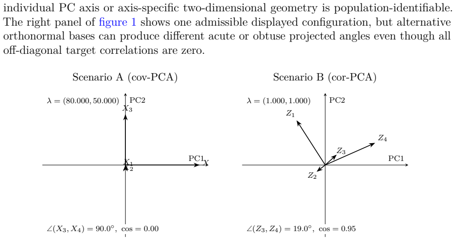
Find one scientific biplot statement that passes all three declared conditions target alignment, spectral identifiability, and Delta_J(C) <= tau yet is demonstrably false about the target matrix's geometry, and the sufficiency of the admissibility criterion collapses. A concrete starting point is to recompute Scenario E from the given correlation matrix R_E: the PC1-PC2 projected angle between Z3 and Z4 is 0 degrees while the full target angle is 60 degrees, so the diagnostic must be checked against the full relationship before any angular claim is retained.
If this is right
- Applied PCA reports should name the target, the spectral object, the displayed components, and the tolerance, not just loadings and percent variance; otherwise the sentence is not auditable.
- Correlation-PCA remains legitimate when the claim is explicitly about standardised association and the subspaces used are identifiable; the silent transfer of a raw-scale claim to a standardised display is what the framework rules out.
- Biplots with repeated or near-repeated eigenvalues cannot support named-axis narratives; they must be rephrased as invariant-subspace statements.
- High retained inertia does not guarantee that the specific pairwise relationships a claim relies on are preserved, so reporting inertia alone is not enough.
- The framework is conditional and population-level; bootstrap stability can accompany but not replace target specification and population diagnosis.
Where Pith is reading between the lines
- The same three-way structure target, identifiability, projection could be carried over to other unsupervised displays such as factor analysis or correspondence analysis, where preprocessing choices, rotational indeterminacy, and truncation create the same gap between computation and claim.
- Because the tolerance tau must be justified before the plot is used as evidence, the framework implicitly pressures researchers toward pre-registering their target and tolerance, or at least disclosing whether the claim was formed after viewing the display.
- A natural extension is a sample-level decision rule: use bootstrap confidence intervals for E_max(J; P) and flag any pairwise error whose upper bound exceeds tau, converting the population inequality into an operational diagnostic.
- The residual-Gram bound suggests a simple reporting addition: alongside the biplot, report the worst pairwise omitted-inner-product error; variable pairs whose bound exceeds the declared tolerance should be visually flagged so the reader knows where the plane cannot be trusted.
Editorial analysis
A structured set of objections, weighed in public.
Referee Report
Summary. The paper proposes a claim-specific admissibility framework for PCA biplots. It separates three conditions: target alignment (the declared scientific target must justify the operator actually diagonalised), spectral identifiability (the invoked axis or invariant subspace must be uniquely determined by the target at the level claimed), and projection adequacy (the displayed projection must preserve the prespecified variable-pair relationships within a scientifically justified tolerance). Claims are formalized as a tuple (Definition 2), projector-based diagnostics are introduced for repeated-eigenvalue blocks, and a residual-Gram bound controls pairwise error from omitted coordinates (Theorem 1). Six exact population scenarios illustrate target shift under standardisation, isotropy-induced non-identifiability, and projection collapse of a 60-degree relationship to 0 degrees. The paper concludes that computational correctness is necessary but not sufficient for scientific interpretability and provides a decision procedure for retaining, reformulating, qualifying, or rejecting a claim.
Significance. If the framework is accepted within its intended scope, it provides a reproducible protocol for auditing PCA-biplot interpretations, with the strength that the population scenarios are exactly constructed and the projector formulation correctly separates axis-level from subspace-level claims. The residual-Gram bound is a clean way to quantify omitted-coordinate distortion for pairwise variable relationships. The paper is also strong on reproducibility: the main scenarios are supported by R/Python workflows and archived materials, and the authors explicitly acknowledge that sampling inference and finite-sample calibration are separate tasks. The central weakness is that the abstract and several general statements claim coverage for 'a PCA-biplot claim' broadly, while the formalism and all operational criteria are developed only for variable-pair relationships under the variable principal coordinate convention; this scope mismatch is load-bearing for the central claim as stated.
major comments (2)
- [Abstract; §2.2 (Definitions 2–3)] The central 'only when' assertion is stated for 'a PCA-biplot claim' generally, but Definition 2 restricts the audited content to P, a set of variable pairs/contrasts, and Definition 3(iii) checks only max_{(j,k)∈P} d(r_{jk}^{(J,B)}(M), r_{jk}(M)). Observation-score interpretations—PC1 group separation, ordering/distances of observations, cluster readings—cannot be encoded in P; for them condition (iii) is undefined or may fail while the score-based claim is fully supported. The framework is sound for variable-pair claims but does not support the unqualified central claim. Restrict the scope in the abstract and conclusions, or extend the framework with a score-space projection-adequacy condition (e.g., comparing full versus displayed differences in principal-component scores for the named contrasts) and illustrate it on the scenarios.
- [§2.4; §3.1] All operational formulas for projection adequacy assume variable principal coordinates (the projected Gram matrix K_J = G_J G_J^T; the coordinate formula v_j^{(a,b)} = (sqrt(λ_a) q_{ja}, sqrt(λ_b) q_{jb})). Definition 2 allows an arbitrary biplot convention B, and the central claim is unqualified, but no convention-specific definition of r^{(J,B)} is given for row-principal, column-principal, or symmetric biplots. A user following the protocol with another convention currently has no well-defined projection-adequacy check. Please either state explicitly that the framework applies only to variable principal coordinates, or supply the general mapping from B to the displayed relationship being audited.
minor comments (4)
- [§2.2] The tuple C = (T,M,O,J,B,P,r,d,τ) is notation-heavy and used mostly as a bookkeeping device. A table of symbols and a short worked example of how to instantiate the tuple for a real claim would improve readability.
- [Theorem 1] The proof is deferred entirely to Supplementary Material SM4. Since Theorem 1 underlies the projector-based diagnostics and the residual bound, a short proof sketch in the main text would help the reader who does not consult the supplement.
- [§2.4] The definition of e^{rel}_{jk}(J) divides by sqrt(M_{jj} M_{kk}); the zero-denominator case is mentioned only informally. Please state explicitly what is reported when one or both marginal variances are zero.
- [Figure 1] In the Scenario A panel, X1 and X2 coincide at the origin; the caption uses 'X1X2' without explanation. A note such as 'X1 and X2 are located at the origin in this plane' would avoid confusion.
Circularity Check
Central 'only when' is a disclosed definitional stipulation; no fitted inputs or self-citations.
specific steps
-
self definitional
[Section 2.2, Definition 3 and 'Claim-specific representational status'; cf. Abstract]
"Conditional on the declared (T,B,P,r,d,τ), the claim C is population-admissible when: (i) target alignment: the invariances and scale encoded by T justify M; (ii) spectral identifiability: the projector O is uniquely determined by M at the level invoked by the claim; (iii) projection adequacy: ΔJ(C) = max_(j,k)∈P d{r(J,B)_jk(M), r_jk(M)} ≤ τ. ... a population-admissible claim is representationally well posed; if any condition fails, it is representationally ill posed for that interpretation."
Representational well-posedness is stipulated to be exactly the conjunction of conditions (i)-(iii), so the abstract's 'only when' assertion is entailed by the definition rather than derived from data or from an independent external criterion. A claim failing any condition is ill posed by construction. The paper discloses this conditionality ('The word conditional is essential...') and fits no parameters, so the circularity is a mild, transparent definitional stipulation rather than a hidden prediction.
full rationale
The paper is a definitional/normative framework rather than a fitted-derivation paper. No parameters are estimated from data; the six controlled scenarios are exact population constructions chosen to illustrate the definitions. Theorem 1 (basis-invariant spectral representation and residual-Gram bound) is a standard consequence of the spectral decomposition and the Cauchy-Schwarz inequality, with its proof delegated to SM4, and it does not presuppose the admissibility verdicts. The reference list contains no self-citations by Pinto and Dias, so the self-citation and imported-uniqueness patterns do not arise. The only circular flavor is that representational well-posedness is defined in Definition 3 as the conjunction of target alignment, spectral identifiability, and projection adequacy, making the central 'only when' true by construction; this is explicitly conditional on a declared target and tolerance and is disclosed in the text. The skeptic's scope concern—that Definition 2 encodes only variable-pair claims under the variable principal-coordinate convention, not score-based or cluster-separation interpretations—is a scope/correctness objection rather than a circularity, and does not increase the circularity score. Overall, the mathematical content is self-contained and the framework is honestly labeled as conditional, so the score is low: 2 reflects one mild definitional stipulation at the core of the claim.
Axiom & Free-Parameter Ledger
free parameters (1)
- Tolerance τ =
none (user-chosen)
axioms (4)
- standard math Spectral theorem for real symmetric positive-semidefinite matrices: M = QΛQ⊤
- standard math Cauchy-Schwarz inequality applied to the positive-semidefinite omitted matrix HJ
- domain assumption Scientific biplot claims can be encoded by a declared target M, a pair set P, and variable principal coordinates
- domain assumption Population-level target matrices are the appropriate audit object, with sampling inference deferred
read the original abstract
Unit-variance standardisation is often applied routinely before principal component analysis (PCA), although it replaces covariance geometry by correlation geometry. A resulting biplot may be computed correctly yet fail to support a scientific interpretation about the original-scale phenomenon. We therefore make the scientific statement, rather than the decomposition alone, the unit of methodological assessment. A PCA-biplot claim is representationally well posed only when the declared scientific target justifies the operator analysed, the invoked axis or invariant subspace is identifiable at the stated level, and the displayed projection preserves the prespecified relationships within a substantively justified tolerance; failure of any condition makes the claim ill posed for the stated interpretation. A projector formulation yields basis-invariant diagnoses for repeated-eigenvalue blocks, and a residual-Gram bound quantifies pairwise error from omitted coordinates. Six controlled population scenarios provide exact representational truth, including zero target association with arbitrary projected angles, collapse of a full-space 60-degree relationship to 0 degrees, and non-identifiable named axes. The contribution is not another reminder that scaling matters: it establishes that computational correctness is necessary but not sufficient for scientific interpretability and provides a formal procedure for retaining, reformulating, qualifying, or rejecting a PCA-biplot statement. A real-data illustration and bootstrap extension are provided as supplementary material.
Figures


Reference graph
Works this paper leans on
-
[1]
Abdi, H. and Williams, L. J. (2010). Principal component analysis. Wiley Interdisciplinary Reviews: Computational Statistics, 2(4), 433--459. Available at: https://doi.org/10.1002/wics.101
doi:10.1002/wics.101 2010
-
[2]
Anderson, T. W. (1963). Asymptotic theory for principal component analysis. The Annals of Mathematical Statistics, 34(1), 122--148. Available at: https://doi.org/10.1214/aoms/1177704248
arXiv 1963
-
[3]
Brereton, R. G. (2025). Principal component analysis: Standardisation. Journal of Chemometrics, 39(1), e3607. Available at: https://doi.org/10.1002/cem.3607
-
[4]
Bro, R. and Smilde, A. K. (2003). Centering and scaling in component analysis. Journal of Chemometrics, 17(1), 16--33. Available at: https://doi.org/10.1002/cem.773
-
[5]
Davis, C. and Kahan, W. M. (1970). The rotation of eigenvectors by a perturbation. III. SIAM Journal on Numerical Analysis, 7(1), 1--46. Available at: https://doi.org/10.1137/0707001
doi:10.1137/0707001 1970
-
[6]
Fisher, R. A. (1936). The use of multiple measurements in taxonomic problems. Annals of Eugenics, 7, 179--188. doi:10.1111/j.1469-1809.1936.tb02137.x
arXiv 1936
-
[7]
Forkman, J. (2019). Hypothesis tests for principal component analysis when variables are standardized. Journal of Agricultural, Biological and Environmental Statistics, 24, 603--622. Available at: https://doi.org/10.1007/s13253-019-00355-5
-
[8]
Gabriel, K. R. (1971). The biplot graphic display of matrices with application to principal component analysis. Biometrika, 58(3), 453--467. Available at: https://doi.org/10.1093/biomet/58.3.453
-
[9]
Gower, J. C. and Hand, D. J. (1996). Biplots. Chapman & Hall, London
1996
-
[10]
Gower, J. C., Le Roux, N. J., and Gardner-Lubbe, S. (2015). Biplots: Quantitative data. Wiley Interdisciplinary Reviews: Computational Statistics, 7(1), 42--62. Available at: https://doi.org/10.1002/wics.1338
-
[11]
Graffelman, J. (2025). Biplots for the correlation matrix. Journal of Computational and Graphical Statistics, 34(4), 1591--1600. Available at: https://doi.org/10.1080/10618600.2025.2469757. Published online 16 April 2025
arXiv 2025
-
[12]
Graffelman, J. and De Leeuw, J. (2023). Improved approximation and visualization of the correlation matrix. The American Statistician, 77(4), 432--442. Available at: https://doi.org/10.1080/00031305.2023.2186952
Pith/arXiv arXiv 2023
-
[13]
Greenacre, M. (2010). Biplots in Practice. Fundaci\'on BBVA, Bilbao
2010
-
[14]
Greenacre, M. J. (2012). Biplots: The joy of singular value decomposition. Wiley Interdisciplinary Reviews: Computational Statistics, 4(4), 399--406. Available at: https://doi.org/10.1002/wics.1200
-
[15]
F., Black, W
Hair, J. F., Black, W. C., Babin, B. J., and Anderson, R. E. (2010). Multivariate Data Analysis, 7th edition. Pearson, Upper Saddle River, NJ
2010
-
[16]
Harris, C. R., Millman, K. J., van der Walt, S. J., et al. (2020). Array programming with NumPy. Nature, 585, 357--362. doi:10.1038/s41586-020-2649-2
-
[17]
Hotelling, H. (1933). Analysis of a complex of statistical variables into principal components. Journal of Educational Psychology, 24(6), 417--441. Available at: https://doi.org/10.1037/h0071325
doi:10.1037/h0071325 1933
-
[18]
Hunter, J. D. (2007). Matplotlib: A 2D graphics environment. Computing in Science & Engineering, 9, 90--95. doi:10.1109/MCSE.2007.55
-
[19]
Jackson, J. E. (1991). A User's Guide to Principal Components. Wiley, New York
1991
-
[20]
Johnson, R. A. and Wichern, D. W. (2007). Applied Multivariate Statistical Analysis, 6th edition. Pearson Prentice Hall, Upper Saddle River, NJ
2007
-
[21]
Jolliffe, I. T. (1989). Rotation of ill-defined principal components. Journal of the Royal Statistical Society: Series C (Applied Statistics), 38(1), 139--147. Available at: https://doi.org/10.2307/2347688
-
[22]
Jolliffe, I. T. (2002). Principal Component Analysis. Springer, New York, 2nd edition
2002
-
[23]
Jolliffe, I. T. and Cadima, J. (2016). Principal component analysis: A review and recent developments. Philosophical Transactions of the Royal Society A, 374(2065), 20150202. Available at: https://doi.org/10.1098/rsta.2015.0202
arXiv 2016
-
[24]
Koltchinskii, V. and Lounici, K. (2017). Normal approximation and concentration of spectral projectors of sample covariance. The Annals of Statistics, 45(1), 121--157. Available at: https://doi.org/10.1214/16-AOS2437
-
[25]
Manly, B. F. J. (2005). Multivariate Statistical Methods: A Primer, 3rd edition. Chapman & Hall/CRC, Boca Raton, FL
2005
-
[26]
McKinney, W. (2010). Data structures for statistical computing in Python. In Proceedings of the 9th Python in Science Conference, 56--61. doi:10.25080/Majora-92bf1922-00a
-
[27]
North, G. R., Bell, T. L., Cahalan, R. F., and Moeng, F. J. (1982). Sampling errors in the estimation of empirical orthogonal functions. Monthly Weather Review, 110(7), 699--706. Available at: https://doi.org/10.1175/1520-0493(1982)110<0699:SEITEO>2.0.CO;2
-
[28]
Python Language Reference, Version 3.13.5
Python Software Foundation (2026). Python Language Reference, Version 3.13.5. Python Software Foundation, Wilmington, Delaware. https://www.python.org/
2026
-
[29]
R Core Team. (2024). R: A Language and Environment for Statistical Computing. R Foundation for Statistical Computing, Vienna, Austria. https://www.R-project.org/
2024
-
[30]
Rencher, A. C. (2002). Methods of Multivariate Analysis, 2nd edition. Wiley, New York
2002
-
[31]
Stewart, G. W. and Sun, J.-G. (1990). Matrix Perturbation Theory. Academic Press, Boston
1990
-
[32]
Tukey, J. W. (1977). Exploratory Data Analysis. Addison--Wesley, Reading, MA
1977
-
[33]
van den Berg, R. A., Hoefsloot, H. C. J., Westerhuis, J. A., Smilde, A. K., and van der Werf, M. J. (2006). Centering, scaling, and transformations: Improving the biological information content of metabolomics data. BMC Genomics, 7, 142. Available at: https://doi.org/10.1186/1471-2164-7-142
-
[34]
Wedin, P.-A. (1972). Perturbation bounds in connection with singular value decomposition. BIT, 12(1), 99--111. Available at: https://doi.org/10.1007/BF01932678
-
[35]
Wold, S., Esbensen, K., and Geladi, P. (1987). Principal component analysis. Chemometrics and Intelligent Laboratory Systems, 2(1--3), 37--52. Available at: https://doi.org/10.1016/0169-7439(87)80084-9
-
[36]
Yu, Y., Wang, T., and Samworth, R. J. (2015). A useful variant of the Davis--Kahan theorem for statisticians. Biometrika, 102(2), 315--323. Available at: https://doi.org/10.1093/biomet/asv008
discussion (0)
Sign in with ORCID, Apple, or X to comment. Anyone can read and Pith papers without signing in.