REVIEW 3 major objections 2 minor 18 references
Differential equations for the recurrence coefficients limits for multiple orthogonal polynomials from a Nevai class
T0 review · 3 major / 2 minor · reviewed 2026-08-14 · deepseek-v4-flash
Pith's one-line read This paper proves that ray limits of nearest-neighbor recurrence coefficients in a multiple Nevai class satisfy an explicit system of $2d(d-1)$ differential equations, which for two measures becomes ordinary.
desk verdict Useful conditional PDE/ODE description of NNRR coefficient limits, with an honest but load-bearing uniform-rate assumption that is unproved at the boundary for the main example class. read the letter →
The pith
A machine-rendered reading of the paper's core claim, the machinery that carries it, and where it could break.
The reading
What carries the argument
The load-bearing object is the piecewise-multilinear interpolant $A_j^{(m)}$ (and its analogue $B_j^{(m)}$) built from all coefficients $a_{\vec n,j}$ with $|\vec n|=m$; it is linear along coordinate axes on each cube and continuous across faces. Lemma 1 shows that under the uniform $o(1/m)$ rate and piecewise $C^1$ regularity, the partial derivatives of the interpolants converge to those of the limits, uniformly on small neighbourhoods. That derivative control makes the first-order Taylor expansion (2.17) of the compatibility conditions (1.8)--(1.10) uniform, so the discrete identities survive passage to the limit and become (2.7)--(2.9). In the Angelesco case, the same limits are described by the rational functions $\Upsilon_i$ on a genus-zero $(d+1)$-sheeted Riemann surface $R_{\vec t}$, and a parametrization of that surface gives explicit formulas (4.9) and the boundary data used in Theorem 4.
What would settle it
For a fixed two-interval Angelesco system, integrate the ODE system (3.5) with the boundary conditions (3.6)--(3.7) and compare it with the recurrence coefficients obtained by iterating the compatibility relations (1.5)--(1.7) to large $|\vec n|$; any visible disagreement between the ODE curve and the recursion data would settle that the differential-equation description is wrong. Conversely, checking whether $m\sup_{\vec s}|A_j^{(m)}(\vec s)-A_j(\vec s)|$ stays bounded as $m\to\infty$ would decide whether the rate hypothesis holds at the boundary.
Extended reading notes
Core claim
The paper's central claim, stated as Theorem 3, is that for any perfect system in the multiple Nevai class whose approximations converge at the uniform rate (2.5)--(2.6), the limiting functions $A_j$ and $B_j$ defined by (2.2)--(2.3) satisfy the identities $\nabla B_i\cdot(\vec\delta_j-\vec s)=\nabla B_j\cdot(\vec\delta_i-\vec s)$, $B_j\nabla B_j\cdot(\vec\delta_i-\vec s)-B_i\nabla B_i\cdot(\vec\delta_j-\vec s)=(\sum_l\nabla A_l)\cdot(\vec\delta_j-\vec\delta_i)$, and $A_j\nabla(B_i-B_j)\cdot(\vec s-\vec\delta_j)+(B_i-B_j)\nabla A_j\cdot(\vec\delta_i-\vec s)=0$ for all pairs. For $d=2$ these reduce to the $3\times3$ ODE system (3.3), and for Angelesco systems to the reduced system (3.5) with the boundary conditions (3.6)--(3.7); the functions are constant on the plateau interval $[c_1,c_2]$ where the pushing effect keeps the extremal support away from an interval.
Load-bearing premise
The theorem stands on the uniform convergence rate $|A_j^{(m)}(\vec s)-A_j(\vec s)|\le o(1/m)$ and the same for $B_j$ on the entire simplex, a rate that for Angelesco systems is presently known only on compact subsets of the interior, with boundary extension open.
Editorial extensions
If this is right
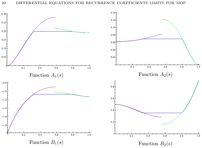
- For $d=2$, computing the limits of all four recurrence coefficients reduces to solving a boundary-value problem for two first-order ODEs, with the plateau interval $[c_1,c_2]$ determined by the support of the equilibrium measure.
- For Angelesco systems, the boundary values (3.6)--(3.7) are closed expressions in the interval endpoints, so the ODE solution is a direct numerical route to the limiting coefficients.
- The three methods compared in the paper---recursive computation of the coefficients, numerical solution of the ODE, and the algebraic-geometric formulas---agree to plotting accuracy, confirming the derived equations on explicit examples.
- For $d>2$, Theorem 3 gives a system of $2d(d-1)$ PDEs as the continuum description of the lattice, connecting the asymptotic theory of multiple orthogonal polynomials to PDE boundary-value problems.
Reading between the lines
- A natural extension, not pursued in the paper, is to relax the uniform $o(1/m)$ rate; the Taylor argument only needs the scaled error to vanish, so rates like $O(m^{-1}\log m)$ may suffice and would make the theorem applicable to broader classes.
- The PDE system can be read as the continuum limit of the discrete integrable system (1.8)--(1.10); this suggests the limiting equations may themselves be integrable or admit hydrodynamic-type reductions, a direction the paper does not discuss.
- For $d>2$, boundary conditions are not yet known; deriving them from endpoint Nevai data, as done here for $d=2$, is a concrete next problem.
- Because the same nearest-neighbor scheme underlies random-matrix ensembles associated with multiple orthogonal polynomials, the ODE description could give a fast way to compute the mean fields in those ensembles, but this is only a speculation.
Signed reviews
Editorial analysis
A structured set of objections, weighed in public.
Referee Report
Summary. The paper studies continuum limits of the nearest-neighbor recurrence coefficients for multiple orthogonal polynomials along rays of the multi-index lattice. It defines a multiple Nevai class in which the limits A_j and B_j of the recurrence coefficients exist along every direction, constructs piecewise multilinear interpolants A_j^(m), B_j^(m) from the coefficients on |n|=m, and proves Theorem 3: if the limiting functions are piecewise C^1 and the interpolants converge uniformly at rate o(1/m) on the whole simplex S^{d-1}, then the limiting functions satisfy the 2d(d-1) partial differential equations (2.7)-(2.9). For d=2 the PDE system reduces to the ODE system (3.3), and for Angelesco systems the authors derive boundary conditions (3.6)-(3.7) from the algebraic-geometric parametrization of the Riemann surface in Section 4. The paper closes with numerical comparisons of three methods for computing the limits in the Angelesco case.
Significance. If the hypotheses hold, the paper gives a new structural description of the continuum limits of nearest-neighbor recurrence coefficients for multiple orthogonal polynomials, connecting discrete integrable systems to PDEs/ODEs. The derivation from the compatibility conditions (1.8)-(1.10) is explicit and transparent, and the d=2 reduction together with the algebraic-geometric parametrization is elegant. The numerical evidence in Section 5 is strong. The main caveat is that the central theorem is conditional on the uniform rate assumption (2.5)-(2.6), which the authors themselves state is open at the boundary for the motivating Angelesco systems; the proof of Theorem 3 as written also does not handle boundary points. These issues are load-bearing for the general claim but appear repairable, and the interior statement is already meaningful.
major comments (3)
- [Section 2.1 and Theorem 3, Eqs. (2.4)-(2.6)] The construction of the approximating functions A_j^(m) and B_j^(m) sets the grid values at points of (1/m)Z_+^{d-1} outside the simplex S^{d-1} to zero. For d>=3 this is incompatible with the uniform convergence assumed in (2.5)-(2.6) on the whole simplex, in particular on the face |s|=1. An axis-parallel cube of side 1/m containing a point s on that face has a vertex outside S^{d-1}; that vertex receives value zero, and in the multilinear interpolation (2.4) its weight can be bounded away from zero and can oscillate with m. Consequently A^(m)(s) need not converge to A_j(s) at all for nonzero boundary values, so the main theorem's hypothesis (ii) is not a harmless regularity condition for the functions defined in Section 2.1. The authors should either clip the interpolation to the simplex, define boundary values differently, or state Theorem 3 on the interior only.
- [Section 2.3, Lemma 1] The proof of Lemma 1 chooses a Euclidean cube centered at s_0 and contained in D_i. Such a cube exists only when s_0 is in the Euclidean interior of S^{d-1}. For points on the boundary of the simplex the argument does not apply, so the proof of Theorem 3 does not cover the boundary even if the uniform rate condition (2.5)-(2.6) holds. Since Theorem 3 is stated for all s in S^{d-1}, the statement should either be restricted to interior points or an independent boundary argument should be supplied.
- [Section 2.2, remark after Theorem 3] The uniform rate condition (ii) is the load-bearing assumption: it is used in Lemma 1 and in the Taylor step (2.17) to pass from the discrete compatibility equations to the PDE system. The definition of the multiple Nevai class only gives pointwise convergence of the recurrence coefficients, not the uniform o(1/m) rate for the interpolants. The authors' own remark states that for Angelesco systems (ii) is known only uniformly on compact subsets of Int(S^{d-1}) and that the boundary case is open. Since Angelesco systems are the principal example class, the main theorem currently applies unconditionally only in the interior. The paper should either prove (ii) for the Angelesco case on the boundary or reformulate the main results with the interior restriction and discuss boundary behaviour separately.
minor comments (2)
- [Section 2.4, proof of Theorem 3] In the justification of uniformity after Eq. (2.17), the text says 'we used (ii) of Theorem 4 and Lemma 1'; the reference should be to condition (ii) of Theorem 3, not Theorem 4.
- [Section 2.3, Lemma 1] In the proof of Lemma 1, the sentence 'By the construction, K belongs to Di' is not automatic for d>2: the cube K of side 1/m containing s can extend outside the neighbourhood U unless M is chosen sufficiently large relative to the dimension. This is easily fixed by enlarging M, but the proof should state the required dependence.
Circularity Check
No significant circularity: the PDE/ODE system is derived from the exact discrete compatibility conditions under explicit rate assumptions, with boundary values supplied independently.
full rationale
The paper's central claim, Theorem 3, derives differential equations for the limiting functions A_j and B_j from the discrete compatibility conditions (1.8)–(1.10) by constructing piecewise-linear approximations, controlling their derivatives via Lemma 1 under the explicit uniform rate hypothesis (2.5)–(2.6), and then passing to the limit through a Taylor expansion. The limiting functions are defined as limits of the actual recurrence coefficients (2.2)–(2.3), not via the differential equations, so the conclusion is not fed back into the derivation. Assumptions (i) and (ii) are explicit hypotheses, not consequences of the PDE system; the authors state plainly that for Angelesco systems the uniform rate (ii) is known only on compact subsets of the interior and that boundary extension is open. This is an honest rigor limitation, not circularity. The d=2 boundary conditions in Theorem 4 are obtained from Weyl's theorem on the scalar Nevai class and from the independent Riemann-surface parametrization of Section 4, which relies on the cited Theorem 5 and on prior algebraic-geometric results; these are external, non-circular inputs. The numerical comparison in Section 5 validates three independent methods (recurrence computation, ODE solution, algebraic-geometric formulas) and agrees, so the ODE system is not fitted to the numerical data. Self-citations appear (e.g., Theorem 2 from [2]), but they are used to establish the Nevai-class membership of Angelesco systems and to provide explicit limits, not as a basis for the differential equations themselves, which are derived from the discrete relations in the present paper. No fitted parameter is renamed as a prediction, no ansatz is smuggled in via citation, and no known result is merely renamed. The chain from discrete compatibility to the differential system is self-contained given its stated assumptions.
Assumptions & free parameters
assumptions (5)
- domain assumption The system of measures is perfect, so the nearest-neighbor recurrence (1.4) and compatibility conditions (1.5)-(1.10) hold for all multi-indices.
- ad hoc to paper The limiting functions A_j and B_j are piecewise C^1 on S^{d-1} and satisfy the uniform o(1/m) approximation bounds (2.5)-(2.6) on the whole simplex.
- domain assumption Theorem 2 of [2]: for Angelesco systems with holomorphic nonvanishing densities, the ray limits of recurrence coefficients exist and are given by the residues of the functions Y_i on the genus-zero Riemann surface R_t.
- standard math Theorem 5 of [5,12,13]: the three-sheeted Riemann surface with four branch points is parametrized by (4.3)-(4.8), giving a diffeomorphism between the half-strip and the branch points.
- standard math Support characterization from [10]: in the d=2 Angelesco case, the set where all derivatives of the limits vanish is either a single point or an interval [c1,c2] inside (0,1).
Cite this review
Pith. "Pith review of Differential equations for the recurrence coefficients limits for multiple orthogonal polynomials from a Nevai class." pith.science (2026). https://pith.science/paper/OSYKPY7F
@misc{pith2026190804540,
  author       = {Pith},
  title        = {Pith review of: Differential equations for the recurrence coefficients limits for multiple orthogonal polynomials from a Nevai class},
  year         = {2026},
  howpublished = {\url{https://pith.science/paper/OSYKPY7F}},
  note         = {Machine review of arXiv:1908.04540}
}
read the original abstract
A limiting property of the nearest-neighbor recurrence coefficients for multiple orthogonal polynomials from a Nevai class is investigated. Namely, assuming that the nearest-neighbor coefficients have a limit along rays of the lattice, we describe it in terms of the solution of a system of partial differential equations. In the case of two orthogonality measures the differential equation becomes ordinary. For Angelesco systems, the result is illustrated numerically.
Figures

Reference graph
Works this paper leans on
-
[1]
Aptekarev, Spectral Problems of High-Order Recurrences, Amer
A.I. Aptekarev, Spectral Problems of High-Order Recurrences, Amer. Math. Soc. Transl., 233 (2014) 43–61
work page 2014
-
[2]
A. I. Aptekarev, S. A. Denisov, M. L. Yattselev, Self-adjoint Jacobi matrices on trees and multiple orthogonal polynomials, Trans. Amer. Math. Soc., 373 (2) (2020), 875–917
work page 2020
-
[3]
A. I. Aptekarev, M. Derevyagin, W. Van Assche, Discrete integrable systems generated by Hermite– Pade approximants, Nonlinearity, 29 (5) (2016) 1487–1506
work page 2016
-
[4]
A.I. Aptekarev, V. Kalyagin, G. Lopez Lagomasino, I.A. Rocha, On the limit behavior of recurrence coefficients for multiple orthogonal polynomials, J. Approx. Theory 139 (2006) 346–370
work page 2006
-
[5]
A. I. Aptekarev, V. A. Kalyagin, V. G. Lysov, D. N. Toulyakov, Equilibrium of vector potentials and uniformization of the algebraic curves of genus 0, J. Comput. Appl. Math., 233 (3) (2009) 602–616
work page 2009
-
[6]
A. I. Aptekarev, V. A. Kalyagin, E. B. Saff, Higher-order three-term recurrences and asymptotics of multiple orthogonal polynomials, Constr. Approx., 30 (2) (2009) 175–223
work page 2009
-
[7]
A. I. Aptekarev, W. Van Assche, M. L. Yattselev, Hermite-Pad´ e Approximants for a Pair of Cauchy Transforms with Overlapping Symmetric Supports, Communications on Pure and Applied Mathematics, 70 (3) (2017) 444–0510
work page 2017
-
[8]
Global fluctuations for Multiple Orthogonal Polynomial Ensembles
M. Duits, B. Fahs, R. Kozhan, Global fluctuations for Multiple Orthogonal Polynomial Ensembles, preprint, arXiv:1912.04599
work page Pith review arXiv 1912
Show all 18 references
-
[9]
Filipuk, M
G. Filipuk, M. Haneczok, W. Van Assche, Computing recurrence coefficients of multiple orthogonal polynomials, Numerical Algorithms, 70 (3) (2015) 519–543
2015
-
[10]
A. A. Gonchar and E. A. Rakhmanov, On the convergence of simultaneous Pad´ e approximants for systems of functions of Markov type, Proc. Steklov Inst. Math. 157 (1983) 31–50. DIFFERENTIAL EQUATIONS FOR RECURRENCE COEFFICIENTS LIMITS FOR MOP 21
1983
-
[11]
V. A. Kaliaguine, On operators associated with Angelesco systems, East J. Approx. 1 (2) (1995) 157–170
1995
-
[12]
Lysov, D.N
V.G. Lysov, D.N. Tulyakov, On a vector potential theory equilibrium problem with the Angelesco matrix of interaction Proc. Steklov Inst. Math., 298 (2017) 170–200
2017
-
[13]
Lysov, D.N
V.G. Lysov, D.N. Tulyakov, On the Supports of Vector Equilibrium Measures in the Angelesco Problem with Nested Intervals Proc. Steklov Inst. Math., 301 (2018) 180–196, https://doi.org/10.1134/S0081543818040144
2018 doi
-
[14]
Simon, Szeg˝ o’s theorem and its descendants: spectral theory for L2 perturbations of orthogonal polynomials, Princeton University Press, 2011
B. Simon, Szeg˝ o’s theorem and its descendants: spectral theory for L2 perturbations of orthogonal polynomials, Princeton University Press, 2011
2011
-
[15]
Van Assche, Chapter 23, Classical and Quantuum Orthogonal Polynomials in One Variable: in (by M.E.H
W. Van Assche, Chapter 23, Classical and Quantuum Orthogonal Polynomials in One Variable: in (by M.E.H. Ismail), volume 98 of Encyclopedia of Mathematics and its Applications. Cambridge University Press, 2005
2005
-
[16]
Van Assche, Nearest neighbor recurrence relations for multiple orthogonal polynomials, J
W. Van Assche, Nearest neighbor recurrence relations for multiple orthogonal polynomials, J. Ap- prox. Theory 163 (2011) 1427–1448
2011
-
[17]
Van Assche, Ratio asymptotics for multiple orthogonal polynomials, In Modern trends in con- structive function theory, Contemp
W. Van Assche, Ratio asymptotics for multiple orthogonal polynomials, In Modern trends in con- structive function theory, Contemp. Math., 661 (2016) 73–85, AMS, Providence, RI
2016
-
[18]
Yattselev, Strong asymptotics of Hermite-Pade approximants for Angelesco systems, Canad
M. Yattselev, Strong asymptotics of Hermite-Pade approximants for Angelesco systems, Canad. J. Math., 68 (5) (2016) 1159–1200, http://dx.doi.org/10.4153/CJM-2015-043-3
2016 doi
Reviewed August 14, 2026 · model on record in the stance chip above.
Discussion (0). Continue with ORCID to comment.