REVIEW 2 major objections 5 minor 1 cited by
Conformal Prediction for Hierarchical Data
T0 review · 2 major / 5 minor · reviewed 2026-08-12 · deepseek-v4-flash
Pith's one-line read Projecting predictions onto a hierarchy's coherent subspace makes conformal sets provably smaller while preserving coverage.
desk verdict Genuinely new link between conformal prediction and forecast reconciliation, with honest limitations: the efficiency gains are real but depend on elliptical residuals, not distribution-free. read the letter →
The pith
A machine-rendered reading of the paper's core claim, the machinery that carries it, and where it could break.
The reading
What carries the argument
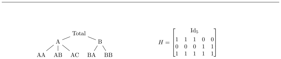
The load-bearing object is the projection matrix onto the coherent subspace Im(H), the set of vectors consistent with the hierarchy's summation constraints. The paper singles out the minimum-trace projection P_{$Σ^{{-1}}$} = H(H^T $Σ^{{-1}}$ H)^{-1} H^T $Σ^{{-1}}$, which is the orthogonal projection in the norm induced by the inverse error covariance, and shows it minimizes the expected weighted sum of squared interval lengths. Two trace inequalities carry the argument: a Pythagorean-type projection inequality for W-norms, and the minimum-trace lemma from forecast reconciliation, which the paper reproves elementarily. Signed vector-valued non-conformity scores are what make the translation from interval lengths to traces work, since centering shifts cancel in the quantile spread.
What would settle it
Generate i.i.d. residuals from a distinctly non-elliptical distribution—for instance, a centered log-normal or a mixture of two Gaussians with different scales—and run Algorithm 4 with the covariance-based projection P_{$Σ^{{-1}}$} against the plain component-wise SCP; if for some component the expected squared interval length is not smaller, or the empirical ratio of lengths departs from the predicted $\sqrt$((P Σ P^T)_{i,i}/Σ_{i,i}) scaling, the elliptical assumption behind Theorem 4 is violated.
Extended reading notes
Core claim
The central discovery is that the reconciliation step translates directly into a scaling law for interval lengths. Because residuals are assumed elliptical, each component's non-conformity score is a scaled version of a single common random variable; after projecting the scores with a matrix P onto the coherent subspace Im(H), the length of component i's interval is $\sqrt$((P Γ P^T)_{i,i}) times a common quantile spread L_α. Expected squared lengths therefore reduce to a trace, and the trace inequality Tr(W P Σ P^T) ≥ Tr(W P_{$Σ^{{-1}}$} Σ P_{$Σ^{{-1}}$}^T) identifies P_{$Σ^{{-1}}$} = H(H^T $Σ^{{-1}}$ H)^{-1} H^T $Σ^{{-1}}$ as the optimal projection for all weight vectors simultaneously. Under i.i.d. residuals with an elliptical distribution admitting a second-order moment, the reconciled procedure run with P_{$Σ^{{-1}}$} gives, for every component, expected squared interval length no larger than that of any other projection onto the coherent subspace, and no larger than the plain component-wise SCP benchmark.
Load-bearing premise
The component-wise efficiency results hold only if the residuals are i.i.d. and follow some elliptical distribution (with unknown shape and parameters); if the residuals are skewed, multimodal, or otherwise non-elliptical, the claimed size reduction can fail, though the coverage guarantees still hold.
Editorial extensions
If this is right
- For any hierarchy and any base regressor, the reconciled ellipsoidal procedure returns prediction regions no larger than the plain ellipsoidal procedure, with no assumptions on the data.
- Component-wise coverage at level 1−α holds for every projection satisfying P H = H, so the efficiency gains never come at the cost of the distribution-free coverage guarantee.
- Under elliptical i.i.d. residuals, the weighted least-squares projection P_w with weights w provably beats the plain component-wise benchmark for the weighted criterion.
- Under additionally bounded second moments, the oracle minimum-trace projection P_{Σ^{-1}} dominates every other projection onto Im(H) and every plain component-wise procedure, simultaneously for all positive weight vectors.
- In simulations, the data-based WLS variant is the most robust improvement over the benchmark, while the MinT variant can degrade for very large hierarchies due to near-singular covariance estimation.
Reading between the lines
- The trace-reduction perspective suggests the same projection approach could be extended to other structured linear constraints beyond summation hierarchies, such as balances in compositional data or linear panel restrictions, with the same proof template.
- The efficiency gain concentrates at the most disaggregated level of the hierarchy in the simulations; a practitioner with primary interest in aggregate nodes might prefer a simpler projection, since aggregated forecasts are already close to coherent.
- The ellipticity assumption, while used only for efficiency, could be tested directly: it predicts that after projection, each component's scores are homothetical—the same distribution up to scale—so a multivariate symmetry test on residuals could flag settings where the claimed dominance may fail.
- Adapting the projection step to the adaptive-conformal-inference framework for non-exchangeable time series, as the authors suggest, would make the size reduction operational in the very applications (energy forecasting) that motivate the hierarchy setup; the coverage side is already covered by ACI, leaving the efficiency side open.
Editorial analysis
A structured set of objections, weighed in public.
Referee Report
Summary. The paper introduces a projection (forecast-reconciliation) step into split conformal prediction for hierarchical multivariate data, where observations satisfy y=H y_{1:n}. For joint coverage, it modifies ellipsoidal conformal prediction by replacing the base regressor with its orthogonal projection onto the coherent subspace in the chosen norm and shows, deterministically, that the resulting ellipsoids have no larger volume. For component-wise coverage, it proposes signed-score split conformal prediction with a projection matrix P satisfying P H=H, proves finite-sample marginal coverage for every component, and then derives efficiency guarantees: under i.i.d. residuals with an elliptical distribution, the projection P_w=H(H^\top diag(w)H)^{-1}H^\top diag(w) achieves no larger expected weighted sum of squared interval lengths than the unprojected benchmark; under a second-order moment, the minimum-trace projection P_{\Sigma^{-1}} dominates every projection onto Im(H) component-wise. The theoretical claims are supported by self-contained proofs in the appendices, and numerical experiments on synthetic hierarchies illustrate the gains and the practical instability of the estimated MinT projection.
Significance. If the stated assumptions are met, the paper contributes one of the few finite-sample efficiency results for conformal prediction and builds a useful bridge between conformal prediction and forecast reconciliation. Its strengths are the transparent decomposition of coverage and efficiency results, the self-contained proofs of the trace inequalities (including an elementary proof of the minimum-trace projection lemma), and the explicit statement of the assumptions under which the efficiency claims hold. The main limitation is also clear: the headline component-wise efficiency result is not distribution-free, since it relies on elliptical residuals and, for Theorem 4, on knowledge of the true covariance matrix. The experiments use Gaussian noise only and show that the estimated MinT projection can underperform the unprojected benchmark in high-dimensional hierarchies, so the empirical evidence does not probe behavior outside Assumption 2.
major comments (2)
- [Section 4, Assumption 1] The statement that residuals are i.i.d. 'in particular when data are i.i.d.' is not correct for the split conformal pipeline. In Algorithms 3-5 the residuals y_t - \hat{\mu}(x_t) for t in D_calib share the regressor \hat{\mu} fitted on D_train, so unconditionally they are exchangeable but generally not independent; a simple counterexample is Gaussian data with a random common mean. The coverage proof of Theorem 2 only needs exchangeability, but the efficiency proofs of Theorems 3 and 4 use order statistics of i.i.d. draws and the common random variable L_alpha, so the i.i.d. assumption is load-bearing for the efficiency claims. The authors should either state Assumption 1 conditionally on the training and estimation data, or separate the exchangeability assumption needed for coverage from the stronger conditional i.i.d. assumption needed for efficiency.
- [Appendix A, proof of Theorem 3 and Lemma 3] Assumption 2 does not require the elliptical residual distribution to have a first-order moment, yet the proof of Theorem 3 centers the residuals by E[\hat{s}_{1,i}], which need not exist; the proof of Theorem 4 even states that Theorem 3 did not rely on a first-order moment, which is contradicted by the written argument. The fix is straightforward: replace the expectation by the location vector c appearing in Definition 3, since interval lengths are translation-invariant and the order-statistic range does not depend on c. The proof should also handle the small-alpha case where the lower quantile index is zero (so L_alpha is infinite) and the case where some diagonal entry of \Gamma is zero, because the factorization E[L_1(C_i)^2] = \Gamma_{i,i} E[L_alpha^2] is not meaningful in those cases without an extended-convention qualification.
minor comments (5)
- [Section 2.3.2] The sentence claiming that signed non-conformity scores between coherent observations and forecasts are also coherent is only true for reconciled forecasts; for an arbitrary base forecast \hat{y}_t, the vector y_t - \hat{y}_t need not lie in Im(H). Please restrict the sentence to the projected scores used in Algorithm 4.
- [Appendix D, Theorem 5] The statement says that Algorithm (2) outputs ellipsoids \check{E} that are more efficient than the ellipsoids \check{E} output by Algorithm (1); the first of these should be \mathring{E}.
- [Section 5 and Appendix F.3.3] The claim that MinT performs worse than the Direct benchmark for the largest hierarchies is clearly supported by Configuration 5 but not by Configuration 6, where the confidence intervals overlap; the wording should be made more cautious.
- [Appendix F] All synthetic residuals are generated as Gaussian, so the experiments do not probe robustness to non-elliptical residual distributions; a sentence stating that the simulations are intended to illustrate the elliptical case and do not validate efficiency outside Assumption 2 would help.
- [Theorem 2, proof in Appendix E.1] The no-tie condition for the upper coverage bound is stated for the vector-valued scores, but the proof needs component-wise distinctness of the univariate scores; full-vector distinctness does not prevent ties in a single component. Please state the condition component-wise.
Circularity Check
No significant circularity: the efficiency results are proven from stated assumptions, with elementary proofs supplied for the cited trace inequalities; self-citations appear only as background.
full rationale
The paper's central derivation chain is self-contained. Theorem 3 and Theorem 4 are proved from Assumptions 1–3 (i.i.d. residuals, elliptical distribution, second-order moment) rather than imported from fitted data. The key structural step is Lemma 3, which shows that marginals of linearly transformed elliptical vectors are homothetic, so all component-wise conformal interval lengths are scalar multiples of one common order-statistic variable L_alpha; this reduces expected squared lengths to diagonal entries of P Gamma P^T. The two trace ingredients, Lemma 5 (fixed-weight trace reduction) and Lemma 1 (minimum-trace projection), are both proved in the appendices, with Lemma 1 receiving an elementary proof of independent interest; thus the central claim does not reduce to an unverified citation. The coverage results are standard exchangeability arguments, and the joint-coverage efficiency result is a deterministic Pythagorean inequality. Cited works involving the authors' own group (Wood et al. 2015 for GAM estimation; Zaffran et al. 2022 in the future-work discussion) are background material and are not load-bearing for any theorem. The elliptical-residual assumption is a stated hypothesis of the efficiency results, not a fitted parameter renamed as a prediction; the paper is explicit that coverage remains distribution-free. Therefore, while the size-dominance claim is conditional on ellipticity—a correctness and robustness consideration rather than circularity—no circular derivation is present.
Assumptions & free parameters
assumptions (4)
- domain assumption Data points (x_t, y_t) are i.i.d., so the non-conformity scores are i.i.d.
- domain assumption The residuals follow an elliptical distribution with unknown parameters.
- domain assumption The residual covariance matrix is positive definite and the second-order moment exists.
- domain assumption The structural matrix H is known and the observed vectors satisfy y = H y_{1:n}.
Cite this review
Pith. "Pith review of Conformal Prediction for Hierarchical Data." pith.science (2026). https://pith.science/paper/OWBNRUWG
@misc{pith2026241113479,
  author       = {Pith},
  title        = {Pith review of: Conformal Prediction for Hierarchical Data},
  year         = {2026},
  howpublished = {\url{https://pith.science/paper/OWBNRUWG}},
  note         = {Machine review of arXiv:2411.13479}
}
read the original abstract
We consider conformal prediction for multivariate data and focus on hierarchical data, where some components are linear combinations of others. Intuitively, the hierarchical structure can be leveraged to reduce the size of prediction regions for the same coverage level. We implement this intuition by including a projection step (also called a reconciliation step) in the split conformal prediction [SCP] procedure, and prove that the resulting prediction regions are indeed globally smaller. We do so both under the classic objective of joint coverage and under a new and challenging task: component-wise coverage, for which efficiency results are more difficult to obtain. The associated strategies and their analyses are based both on the literature of SCP and of forecast reconciliation, which we connect. We also illustrate the theoretical findings, for different scales of hierarchies on simulated data.
Figures


Figures from the paper (1 more)

Forward citations
Cited by 1 Pith paper
-
Multi-Scale Conformal Prediction: A Theoretical Framework with Coverage Guarantees
A multi-scale conformal prediction set formed by intersecting scale-specific sets keeps marginal coverage by a union bound, but the paper's efficiency and asymptotic optimality theorems are not valid.
Reference graph
Works this paper leans on
-
[1]
In this section (as in Appendix A), we restate all the material needed so that this appendix is fully self- contained and may be read without reading back the main body of the article. The proof of Theorem 4 is based on a key equality established in the proof of Theorem 3 and on a minimum-trace-projection result that is central in the theory of forecast r...
work page 2019
-
[2]
We conclude the theoretical part of the appendices with the proofs of the coverage results. They rely on an absolutely standard methodology in the literature of conformal prediction (see, for instance, Tibshirani et al., 25 2019, proof of Theorem 1), with rather immediate adaptations due to the multivariate context and to the choice of signed non-conformi...
work page 2019
-
[3]
Ross Hollyman, Fotios Petropoulos, and Michael E
Preprint, arXiv:2409.18508. Ross Hollyman, Fotios Petropoulos, and Michael E. Tipping. Understanding forecast reconciliation.European Journal of Operational Research, 294(1):149–160,
-
[4]
Tonu Kollo and Dietrich von Rosen.Advanced Multivariate Statistics with Matrices
Preprint, arXiv:2502.03609. Tonu Kollo and Dietrich von Rosen.Advanced Multivariate Statistics with Matrices. Mathematics and Its Applications. Springer,
-
[5]
(2021) relying onPW–projections
is a result of our own though it was inspired by both Lemma 1 and the approach by Panagiotelis et al. (2021) relying onPW–projections. C.3 How we leveraged and transferred these results (and why it was not immediate) On the unnecessity of unbiasedness.As we made clear several times in Section C.2, a key assumption in the literature of forecast reconciliat...
work page 2021
-
[6]
By linearity of a projection, the point forecasts~yare also unbiased
LetP be a projection ontoIm(H)and denote ~y =Pˆy. By linearity of a projection, the point forecasts~yare also unbiased. Since observations are coherent, we have y− ~y def =y−P ˆy=P ( y− ˆy ) =P ˆs def = ~s. The mean-squared error of~yinW–norm thus equals mse (~y,y,W ) =E [ Tr ( W~s~s⊤)] = Tr ( WPE [ˆsˆs⊤] P⊤ ) = Tr ( WPΣP ⊤) . Actually, the formula above ...
work page 2011
-
[7]
Anastasios Panagiotelis, George Athanasopoulos, Puwasala Gamakumara, and Rob J
Preprint, arXiv:2501.19038. Anastasios Panagiotelis, George Athanasopoulos, Puwasala Gamakumara, and Rob J. Hyndman. Forecast reconciliation: A geometric view with new insights on bias correction.International Journal of Forecasting, 37(1):343–359,
-
[8]
Preprint, arXiv:2501.18991. Ryan J. Tibshirani, Rina Foygel Barber, Emmanuel Candes, and Aaditya Ramdas. Conformal prediction under covariate shift. InAdvances in Neural Information Processing Systems (Neurips’2019), volume 32, pp. 2530–2540,
arXiv 2019
Show all 21 references
-
[9]
Margaux Zaffran, Olivier Féron, Yannig Goude, Julie Josse, and Aymeric Dieuleveut
Preprint, arXiv:2403.03850. Margaux Zaffran, Olivier Féron, Yannig Goude, Julie Josse, and Aymeric Dieuleveut. Adaptive conformal predictions for time series. InProceedings of the Thirty-Nitnth International Conference on Machine Learning (ICML’22), volume 162 of PMLR, pp. 258...
-
[10]
A spherical distribution with a second-order moment has a covariance matrix proportional to the identity: there existsσ2∈[0,+∞)such thatE [ zz⊤] =σ 2 Idk. Proof. The first property is proved by considering permutation matricesΓ. The second property holds because u = 0 is the o...
2005
-
[11]
The matrixPw satisfies PwH =H, i.e.,Pw leaves elements ofIm(H)unchanged
in the following sense: E [m∑ i=1 wi L1 (~Ci(xT+1 ) )2 ] ⩽E [m∑ i=1 wi L1 (ˆCi(xT+1 ) )2 ] .(5) Proof. The matrixPw satisfies PwH =H, i.e.,Pw leaves elements ofIm(H)unchanged. Since observations yt are coherent, we have, for allt∈Dcalib, ~st def =y t−P wˆyt =P w ( yt−ˆyt ) =P ...
2021
-
[13]
Lemma 1(Minimum-trace projection, Wickramasuriya et al., 2019).LetW andΣbe two symmetric m×m matrices, whereW is positive semi-definite andΣis positive definite
The latter article sees the minimization problem at hand as a constrained minimization problem (given how projections ontoIm(H)may be written), thus introduced a Lagrangian and discussed Karush-Kuhn-Tucker conditions to solve it. Lemma 1(Minimum-trace projection, Wickramasuriy...
2019
-
[14]
C.1 Brief overview of the literature on forecast reconciliation For a complete review on the forecast reconciliation literature, we refer the reader to Athanasopoulos et al
C Forecast reconciliation: review, connections made, challenges overcome The aim of this appendix is to provide some background on the theory of forecast reconciliation and to explain how we connected it to conformal prediction in the proofs of Appendices A and B. C.1 Brief ov...
2024
-
[17]
Summary of the challenges overcome.In a nutshell, the main challenge overcome was to relate the two minimization problems(12) and (13), and in the first place, state suitably the efficiency criterion(12), which, to the best of our knowledge, is a novel criterion. The main tool...
2022
-
[21]
MatrixAConfig
Coverage-wise, the table below indicates that the nominal joint-coverage of1−α = 90%is achieved irrespective of the algorithm considered or choice of matrixA. MatrixAConfig. Alg. (1) Alg. (2) Idm 1 90%±0.0059% 90%±0.0059% 2 90%±0.0061% 90%±0.0061% Diag(ˆΣ)−1 1 90%±0.0060% 90%±...
2021
-
[103]
= /radicaltp/radicalvertex/radicalvertex√1 103 103 ∑ r=1 ( xr−x103 )2 ,where x103 = 1 103 103 ∑ r=1 xr. Finally, we report in the table below the following point estimates and associated confidence intervals on the underlying unconditional probabilities and expectations: cand ...
2021
-
[2017]
They form a good compromise between forecast efficiency and interpretability
are a popular modeling for many real-world problems, like electricity demand (see Wood et al., 2015). They form a good compromise between forecast efficiency and interpretability. In that setting, univariate response variablesz t based on featuresxt∈R d, wheret∈[T], are expres...
2023
-
[2018]
Signed-error conformal regression
Henrik Linusson, Ulf Johansson, and Tuve Löfström. Signed-error conformal regression. InAdvances in Knowledge Discovery and Data Mining (PAKDD’2014), Part I, volume 8443 ofLecture Notes in Computer Science, pp. 224–236. Springer,
2014
-
[2023]
Preprint, arXiv:2306.06342. 13 J. Lei, Max G’Sell, Alessandro Rinaldo, Ryan J Tibshirani, and Larry Wasserman. Distribution-free predictive inference for regression.Journal of the American Statistical Association, 113(523):1094–1111,
-
[2024]
Robin Dunn, Larry Wasserman, and Aaditya Ramdas
Preprint, arXiv:2403.16336. Robin Dunn, Larry Wasserman, and Aaditya Ramdas. Distribution-free prediction sets for two-layer hierarchical models.Journal of the American Statistical Association, 118(544):2491–2502,
-
[2025]
Margaux Brégère and Malo Huard
Preprint, arXiv:2502.09985. Margaux Brégère and Malo Huard. Online hierarchical forecasting for power consumption data.International Journal of Forecasting, 38(1):339–351,
Reviewed August 12, 2026 · model on record in the stance chip above.
Discussion (0). Continue with ORCID to comment.