REVIEW 4 major objections 5 minor 1 cited by
An Incremental Approach to Online Dynamic Mode Decomposition for Time-Varying Systems with Applications to EEG Data Modeling
T0 review · 4 major / 5 minor · reviewed 2026-08-14 · deepseek-v4-flash
Pith's one-line read Incremental SVD updates let dynamic mode decomposition track time-varying systems online, even when the data matrix is singular.
desk verdict Incremental SVD for online DMD is a sensible incremental step, but the proof has a real gap and the reduced-order claim is unquantified. read the letter →
The pith
A machine-rendered reading of the paper's core claim, the machinery that carries it, and where it could break.
The reading
What carries the argument
The carrying mechanism is the incremental singular value decomposition of a data matrix with a new column appended. For a weighted update, the new SVD factors are obtained from the SVD of the small broken-arrow matrix $S_k=[\Sigma_{xk}\ \rho^{-1}U_{xk}^*x_{k+1}]$, which gives the rank-one correction term $v_{sk,2}\Sigma_{xk+1}^{-1}U_{xk+1}^*$; the windowed version first removes the oldest column with a similar low-rank modification and then appends the newest. The key identity used in both proofs is $U_{xk+1}\Sigma_{xk+1}-\rho U_{xk}\Sigma_{xk}V_{sk,1}=x_{k+1}v_{sk,2}$, which converts the difference between old and new data matrices into the outer product that drives the operator update. This machinery makes the DMD update cost $O(nr+r^3)$ per step for a reduced order $r$, independent of the total data length.
What would settle it
Construct a time-varying linear system with known $A_k$, stream its data through the weighted incremental DMD, and at each step compare the updated operator with the batch least-squares solution recomputed from all stored data; if the truncated update's error grows without bound as the singular-value threshold increases while the batch solution stays accurate, the unquantified truncation step is the cause. A sharper check is numerical: verify whether $U_{xk+1}\Sigma_{xk+1}-\rho U_{xk}\Sigma_{xk}V_{sk,1}=x_{k+1}v_{sk,2}$ still holds when singular values below $\sigma_{\mathrm{thr}}$ are discarded.
Extended reading notes
Core claim
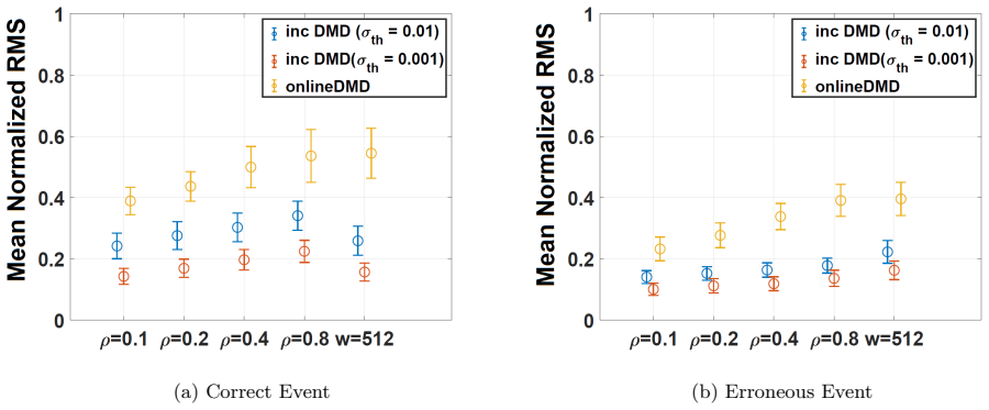
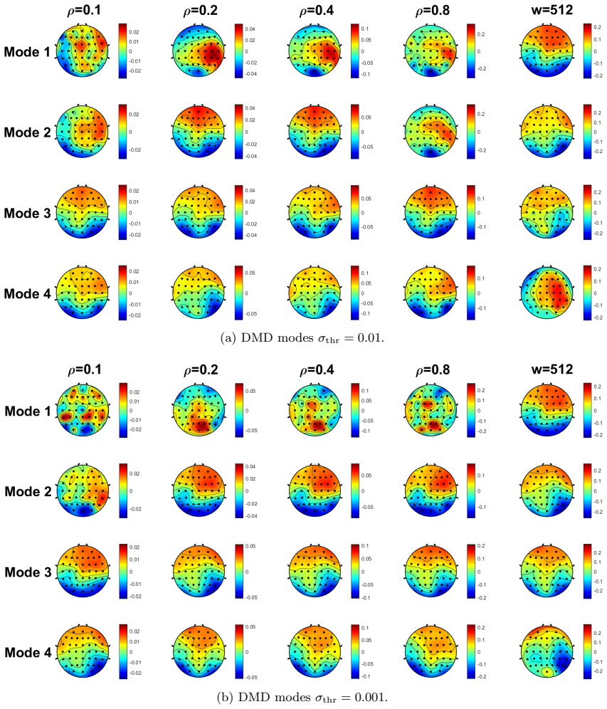
The paper claims that the time-varying DMD operator can be updated in rank-one form: $A_{k+1}=A_k+(y_{k+1}-A_k x_{k+1})v_{sk,2}\Sigma_{xk+1}^{-1}U_{xk+1}^*$, where the correction term comes from the incremental SVD of the augmented data matrix. Because the update is built on the SVD rather than on the inverse covariance, it continues to work when $X_kX_k^*$ is singular, a case where the Sherman-Morrison-based online DMD requires a heuristic initialization. The same construction yields reduced-order projected operators by keeping only singular values above a threshold, and analogous updates for the pair $(A_k,B_k)$ in DMD with control. On preprocessed EEG data, the SVD-based algorithms reconstruct and predict error-related potentials with lower normalized RMS error than the online DMD baseline, and the dominant DMD modes align with frontal-lobe activity during erroneous events.
Load-bearing premise
The load-bearing premise is that, after truncating the SVD to the leading $r$ singular values, the exact algebraic identity used to derive the rank-one update still holds closely enough that the resulting reduced-order DMD operator is accurate; the paper provides no error bound linking the truncation threshold to operator error (equations (33) and (38)).
Editorial extensions
If this is right
- A streaming implementation can maintain a time-varying DMD model without storing the full data matrix, using only the current operator and the incremental SVD factors.
- The algorithm keeps working when the data covariance is singular, a regime where Sherman-Morrison updates need a heuristic pseudo-inverse initialization.
- Users can select or adapt the reduced model order online by thresholding singular values, and the projected operator gives low-dimensional prediction at each time step.
- For systems with known exogenous inputs, the DMDc extension tracks both the dynamics matrix and the input matrix online, with better prediction than ignoring the control term in the paper's numerical example.
- On EEG data, the resulting models capture the time-varying error-related potential and produce dominant spatial modes consistent with frontal-lobe activity.
Reading between the lines
- A testable extension the authors leave implicit: feed the same incremental SVD machinery through a nonlinear observable map (extended DMD style) and compare tracking on the same time-varying systems; the singular-value access would carry over, but the truncation-error question would become more acute.
- The complexity comparison suggests incremental DMD is preferable to Sherman-Morrison online DMD when the reduced order $r$ satisfies $r<n^{2/3}$; for larger $r$, the $O(nr+r^3)$ update may lose that advantage.
- The lack of a bound linking the singular-value threshold to operator error means practitioners must tune $\sigma_{\mathrm{thr}}$ empirically; a natural next step would be a perturbation bound for the truncated update, which would turn the heuristic threshold into a provable accuracy knob.
Signed reviews
Editorial analysis
A structured set of objections, weighed in public.
Referee Report
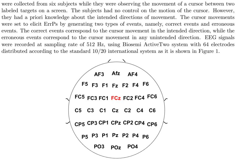
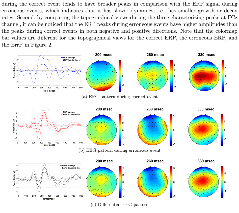
Summary. The paper develops incremental, SVD-based algorithms for online Dynamic Mode Decomposition (DMD) and DMD with control (DMDc) for time-varying systems, in both a weighted (discounted-data) and a sliding-window formulation. The authors derive recursive updates for the least-squares DMD operator from incremental SVD updates, state reduced-order variants obtained by truncating to the leading r singular values, and argue that the approach gives access to time-varying singular values, handles singular data matrices, and avoids storing the data matrix. The autonomous-system algorithms are evaluated on EEG error-related-potential data and compared with the online DMD of [35]; the non-autonomous algorithms are illustrated on randomly generated linear time-varying systems.
Significance. If the full-rank recursion is correct and the reduced-order extension can be rigorously justified, this is a potentially useful streaming DMD method: it avoids storing the data matrix, provides singular values for model-order selection, and can operate when the empirical covariance is singular. The out-of-sample EEG prediction protocol, the comparison with online DMD, and the public MATLAB code are concrete strengths, as is the fact that the full-rank weighted update reduces to a standard recursive least-squares-like correction. The significance is tempered, however, by the absence of any error analysis for the truncated updates and by flaws in the written proofs of the exact updates; both bear directly on the central claim that an 'appropriately reduced model' can be maintained online.
major comments (4)
- [§4, Theorem 1 (Eq. 33) and Theorem 2 (Eq. 38)] The reduced-order update is asserted but not derived from a rank-r least-squares problem. Equations (33) and (38) are obtained by replacing the full SVD factors in the exact recursion (32)/(37) with their leading-r counterparts and replacing A_k by \bar A_k, but this substitution is not exact once a previous truncation has been made: the error from earlier steps is carried forward, and no bound in Theorem 1 or 2 links the threshold \sigma_thr (or the rank r) to either the difference between \bar A_{k+1}^{trunc} and the truncated least-squares operator or to future prediction error. The sentence 'If X_{k+1} is well-approximated by its projection' is an assumption, not a proof of exactness. The same gap appears in the DMDc analogues in Theorems 3 and 4. This is load-bearing for the abstract's claim that the algorithms 'allow us to determine an appropriately reduced model at each time.' I ask the authors either to provide a rigorous error analysis of the truncated recursion or to reframe the reduced-order claims as a heuristic and add experiments that directly quantify the truncation error.
- [Appendix C (Eq. 57) and Appendix D (Eq. 64)] The proofs of the exact updates contain false orthogonality identities. In Appendix C, V_sk = [V_sk,1; v_sk,2] is an (n+1) x n matrix with orthonormal columns, so it satisfies V_sk^* V_sk = I; the step at Eq. (57) uses V_sk,1 V_sk,1^* = I and V_sk,1 v_sk,2^* = 0, which are not implied and are in fact false (for n = 1, V_sk is a unit 2-vector, and V_sk,1 V_sk,1^* = |a|^2 is not 1 unless |a|=1). The same problem appears in Appendix D, where V\'sk V\'sk^* = I and V_hatsk,1 V_hatsk,1^* = I are used even though these matrices are generally projections, not identities, when the number of columns is smaller than the row dimension. The final identities, e.g. Eq. (58), may well be recoverable by a corrected argument starting from S_k V_sk = U_sk \Sigma_sk in the full-rank weighted case, but the written proofs are not valid as they stand and must be rewritten.
- [§4, paragraph after Eq. (39)] The complexity claim 'O(nr + r^3)' and the conclusion that the incremental approach is better when 'r < n^{2/3}' are not justified by the equations in the paper. The update in (32) computes A_k x_{k+1} and adds a rank-one correction to an n x n matrix, which is O(n^2) for a dense A_k; even the projected update (34) requires \bar U_{k+1}^* \bar A_k \bar U_{k+1}, which is not simply the stored reduced operator \tilde A_k unless additional structure is specified. The authors should state exactly which matrices are stored and updated, and give an operation count for those objects, before claiming a complexity advantage over streaming DMD or online DMD.
- [§5, Figures 3–6 and accompanying text] The EEG comparison with online DMD is partly confounded by the baseline's initialization. In the singular-data case, the authors initialize online DMD with the zero matrix and P_init = alpha I, as suggested in [35], so the poor performance of online DMD in Figures 3–5 may reflect this heuristic initialization rather than an intrinsic advantage of the incremental SVD update. The experiment on well-conditioned raw EEG data (Figure 6), where the two methods perform similarly, supports the authors' own explanation that the difference is due to the ill-conditioned dataset, but the text should state this limitation more prominently and avoid presenting the singular-case comparison as a direct algorithmic superiority result.
minor comments (5)
- [§2.4, Eq. (14)] In the windowed cost function (8), the weight of the oldest sample x_{k-w+1} should be rho^{w-1}, not rho^k as written in the displayed definition of X_k; this appears to be a typo that should be fixed for consistency with the subsequent weighted case.
- [§4, Theorem 1 and Theorem 2] The reduced-order quantities \bar v_{sk,2} and \bar v_{\hat sk,2} are not explicitly defined. The authors should specify whether they are the bottom block rows of the right singular vectors of the truncated incremental SVD update, and state the dimensions of all reduced-order factors.
- [§5, Eq. (40)] The symbol y_k is overloaded: it denotes both the recorded EEG value and the arguments of max and min in the denominator. Using different symbols for the bounds would remove ambiguity.
- [Appendix B, Proposition 2] When w < n, the definition q = w is used, but the decremented matrix \'chi_k has w - 1 columns, so its rank can drop below q. The treatment of zero singular values and the dimensions of U_{\'chi_k} in this case is not discussed and should be clarified.
- [§2.2, reduced DMDc formulas] In the display following the definition of the reduced DMDc model, the formula for \tilde B_c uses unbolded V_c(\Sigma_c)^{-1} U_{cb}^* without bars, while the neighboring formulas use barred quantities; this notation should be made consistent.
Circularity Check
No circularity: the incremental DMD updates are algebraic consequences of the least-squares DMD definition, and the EEG predictions are evaluated on future samples not used to fit the model.
full rationale
The paper's core derivations (Theorems 1–4) are self-contained algebraic manipulations of the least-squares DMD / DMDc definitions (Eqs. 15, 18) combined with external incremental SVD updates from Refs. [1,2,26]. The update formulas (32), (37), (43), and (46) are obtained by substituting the incremental SVD factors into the definition of the next DMD operator and simplifying; they do not assume the target result. No fitted parameter is renamed as a prediction: the EEG experiments stream data, update the operator from past and current measurements, and then forecast a 64-sample future window that was not used in the update at that step. The hyperparameters ρ, w, and σthr are selected by the authors, but this is model selection, not a derivation step that reduces to the prediction target. The paper does not rely on self-citation: Ref. [35] (Online DMD) is by different authors, and the incremental SVD machinery comes from independent literature. The main caveats are correctness/approximation concerns rather than circularity: the truncated updates (33) and (38) are asserted by the statement 'If X_{k+1} is well-approximated by its projection' without an error bound linking σthr to DMD operator error, and the proofs of Theorems 1 and 2 contain orthogonality identities (e.g., Vsk,1Vsk,1∗ = I) that are false for the indicated matrix dimensions. These issues undermine the rigor of the reduced-order claim, but they do not make the derivation circular. The derivation is not equivalent to its inputs by construction, and no step reduces a predicted quantity to a fitted parameter.
Assumptions & free parameters
free parameters (4)
- Discount factor rho =
0.1, 0.2, 0.4, 0.8 in EEG experiments; 0.9 in control experiments
- Window length w =
512 samples for EEG; 40 for synthetic DMDc
- Singular value threshold sigma_thr =
0.01 and 0.001 for EEG
- Initial window length w0 =
512 samples, with 128 in Appendix F
assumptions (4)
- domain assumption High-dimensional data are generated by an unknown low-dimensional time-varying linear dynamics.
- ad hoc to paper Truncating the SVD to the leading r singular values leaves the update formula (33) valid without an error term.
- standard math Minimum-norm least-squares solution properties of the reduced SVD hold for singular data matrices.
- domain assumption Preprocessing with CAR and 1-10 Hz band-pass filtering makes the EEG data matrix singular while preserving the ErrP signal.
Cite this review
Pith. "Pith review of An Incremental Approach to Online Dynamic Mode Decomposition for Time-Varying Systems with Applications to EEG Data Modeling." pith.science (2026). https://pith.science/paper/OYUESVQC
@misc{pith2026190801047,
  author       = {Pith},
  title        = {Pith review of: An Incremental Approach to Online Dynamic Mode Decomposition for Time-Varying Systems with Applications to EEG Data Modeling},
  year         = {2026},
  howpublished = {\url{https://pith.science/paper/OYUESVQC}},
  note         = {Machine review of arXiv:1908.01047}
}
read the original abstract
Dynamic Mode Decomposition (DMD) is a data-driven technique to identify a low dimensional linear time invariant dynamics underlying high-dimensional data. For systems in which such underlying low-dimensional dynamics is time-varying, a time-invariant approximation of such dynamics computed through standard DMD techniques may not be appropriate. We focus on DMD techniques for such time-varying systems and develop incremental algorithms for systems without and with exogenous control inputs. We build upon the work in [35] to scenarios in which high dimensional data are governed by low dimensional time-varying dynamics. We consider two classes of algorithms that rely on (i) a discount factor on previous observations, and (ii) a sliding window of observations. Our algorithms leverage existing techniques for incremental singular value decomposition and allow us to determine an appropriately reduced model at each time and are applicable even if data matrix is singular. We apply the developed algorithms for autonomous systems to Electroencephalographic (EEG) data and demonstrate their effectiveness in terms of reconstruction and prediction. Our algorithms for non-autonomous systems are illustrated using randomly generated linear time-varying systems.
Figures
Figures from the paper (13 more)




Forward citations
Cited by 1 Pith paper
-
Online Physics-Informed Dynamic Mode Decomposition: Theory and Applications
OPIDMD combines online proximal gradient descent with physics-informed matrix constraints to learn time-varying linear models of dynamical systems, claiming state-of-the-art short-term prediction on noisy benchmarks.
Reference graph
Works this paper leans on
- [35]
-
[1]
M. Brand, Incremental singular value decomposition of uncertain data with missing values, in European Conference on Computer Vision , Springer, 2002, 707–720
work page 2002
-
[2]
M. Brand, Fast low-rank modifications of the thin singular value decomposition, Linear Algebra and its Applications, 415 (2006), 20–30
work page 2006
-
[3]
B. W. Brunton, L. A. Johnson, J. G. Ojemann and J. N. Kutz, Extracting spatial–temporal coherent patterns in large-scale neural recordings using dynamic mode decomposition, Journal of Neuroscience Methods, 258 (2016), 1–15
work page 2016
-
[4]
R. Chavarriaga and J. D. R. Mill´ an, Learning from EEG error-related potentials in noninvasive brain-computer interfaces, IEEE Transactions on Neural Systems and Rehabilitation Engineering , 18 (2010), 381–388
work page 2010
-
[5]
R. Chavarriaga, A. Sobolewski and J. D. R. Mill´ an, Errare machinale est: The use of error-related potentials in brain-machine interfaces, Frontiers in Neuroscience, 8 (2014), 208
work page 2014
-
[6]
X. Chen and K. S. Candan, LWI-SVD: Low-rank, windowed, incremental singular value decompositions on time- evolving data sets, in Proceedings of the 20th ACM SIGKDD International Conference on Knowledge Discovery and Data Mining , ACM, 2014, 987–996
work page 2014
-
[7]
A. C. Costa, T. Ahamed and G. J. Stephens, Adaptive, locally linear models of complex dynamics, Proceedings of the National Academy of Sciences , 116 (2019), 1501–1510
work page 2019
Show all 35 references
-
[8]
Delorme and S
A. Delorme and S. Makeig, EEGLAB: an open source toolbox for analysis of single-trial eeg dynamics including independent component analysis, Journal of Neuroscience Methods , 134 (2004), 9–21
2004
-
[9]
P. W. Ferrez and J. d. R. Mill´ an, Error-related EEG potentials generated during simulated brain–computer interaction, IEEE Transactions on Biomedical Engineering , 55 (2008), 923–929
2008
-
[10]
Grosek and J
J. Grosek and J. N. Kutz, Dynamic mode decomposition for real-time background/foreground separation in video, arXiv preprint arXiv:1404.7592
-
[11]
Gu and S
M. Gu and S. C. Eisenstat, A stable and fast algorithm for updating the singular value decomposition , Technical Report YALEU/DCS/RR-966, Department of Computer Science, Yale University, New Haven, CT, 1993
1993
-
[12]
Hemati, E
M. Hemati, E. Deem, M. Williams, C. W. Rowley and L. N. Cattafesta, Improving separation control with noise-robust variants of dynamic mode decomposition, in 54th AIAA Aerospace Sciences Meeting, 2016, 1103
2016
-
[13]
M. S. Hemati, M. O. Williams and C. W. Rowley, Dynamic mode decomposition for large and streaming datasets, Physics of Fluids , 26 (2014), 111701
2014
-
[14]
T. K. Huckle, Efficient computation of sparse approximate inverses, Numerical Linear Algebra with Applications, 5 (1998), 57–71
1998
-
[15]
Isermann and M
R. Isermann and M. M¨ unchhof,Identification of Dynamic Systems: An Introduction with Applications , Springer Science & Business Media, 2010
2010
-
[16]
S. M. Kay, Fundamentals of Statistical Signal Processing , Prentice Hall PTR, 1993
1993
-
[17]
B. O. Koopman, Hamiltonian systems and transformation in Hilbert space, Proceedings of the National Academy of Sciences, 17 (1931), 315–318. 34
1931
-
[18]
Korda and I
M. Korda and I. Mezi´ c, Linear predictors for nonlinear dynamical systems: Koopman operator meets model predictive control, Automatica, 93 (2018), 149–160
2018
-
[19]
J. N. Kutz, S. L. Brunton, B. W. Brunton and J. L. Proctor, Dynamic Mode Decomposition: Data-Driven Modeling of Complex Systems , vol. 149, SIAM, 2016
2016
-
[20]
Macesic, N
S. Macesic, N. Crnjaric-Zic and I. Mezic, Koopman operator family spectrum for nonautonomous systems-part 1, arXiv preprint arXiv:1703.07324
-
[21]
Matsumoto and T
D. Matsumoto and T. Indinger, On-the-fly algorithm for dynamic mode decomposition using incremental singular value decomposition and total least squares, arXiv preprint arXiv:1703.11004
-
[22]
C. D. Meyer, Matrix Analysis and Applied Linear Algebra , SIAM, 2001
2001
-
[23]
Mezi´ c, Spectral properties of dynamical systems, model reduction and decompositions, Nonlinear Dynamics, 41 (2005), 309–325
I. Mezi´ c, Spectral properties of dynamical systems, model reduction and decompositions, Nonlinear Dynamics, 41 (2005), 309–325
2005
-
[24]
Mezi´ c, Analysis of fluid fows via spectral properties of the Koopman operator, Annual Review of Fluid Mechanics, 45 (2013), 357–378
I. Mezi´ c, Analysis of fluid fows via spectral properties of the Koopman operator, Annual Review of Fluid Mechanics, 45 (2013), 357–378
2013
-
[25]
Mezi´ c and A
I. Mezi´ c and A. Banaszuk, Comparison of systems with complex behavior, Physica D: Nonlinear Phenomena , 197 (2004), 101–133
2004
-
[26]
G. M. Oxberry, T. Kostova-Vassilevska, W. Arrighi and K. Chand, Limited-memory adaptive snapshot selection for proper orthogonal decomposition, International Journal for Numerical Methods in Engineering , 109 (2017), 198–217
2017
-
[27]
J. L. Proctor, S. L. Brunton and J. N. Kutz, Dynamic mode decomposition with control, SIAM Journal on Applied Dynamical Systems, 15 (2016), 142–161
2016
-
[28]
J. L. Proctor and P. A. Eckhoff, Discovering dynamic patterns from infectious disease data using dynamic mode decomposition, International Health, 7 (2015), 139–145
2015
-
[29]
C. W. Rowley, I. Mezi´ c, S. Bagheri, P. Schlatter and D. S. Henningson, Spectral analysis of nonlinear flows, Journal of Fluid Mechanics , 641 (2009), 115–127
2009
-
[30]
P. J. Schmid, Dynamic mode decomposition of numerical and experimental data, Journal of Fluid Mechanics , 656 (2010), 5–28
2010
-
[31]
Sherman and W
J. Sherman and W. J. Morrison, Adjustment of an inverse matrix corresponding to a change in one element of a given matrix, The Annals of Mathematical Statistics , 21 (1950), 124–127
1950
-
[32]
Surana, Koopman operator based nonlinear dynamic textures, in 2015 American Control Conference (ACC), IEEE, 2015, 1333–1338
A. Surana, Koopman operator based nonlinear dynamic textures, in 2015 American Control Conference (ACC), IEEE, 2015, 1333–1338
2015
-
[33]
J. H. Tu, C. W. Rowley, D. M. Luchtenburg, S. L. Brunton and J. N. Kutz, On dynamic mode decomposition: Theory and applications, Journal of Computational Dynamics , 1 (2014), 391–421
2014
-
[34]
M. O. Williams, I. G. Kevrekidis and C. W. Rowley, A data–driven approximation of the Koopman operator: Extending dynamic mode decomposition, Journal of Nonlinear Science , 25 (2015), 1307–1346
2015
Reviewed August 14, 2026 · model on record in the stance chip above.
Discussion (0). Continue with ORCID to comment.