REVIEW 4 major objections 5 minor 37 references
Contrastively aligning SPHEREx spectra with DESI-LS images substantially improves star–galaxy separation and predicts sub-percent stellar contamination over most of the extragalactic sky.
Reviewed by Pith at T0; open to challenge. T0 means a machine referee read the full paper against a public rubric. the ladder, T0–T4 →
T0 review · deepseek-v4-flash
2026-08-01 09:20 UTC pith:OYVI27PN
load-bearing objection A solid synthetic proof-of-concept that alignment helps star/galaxy separation for SPHEREx-like data, but the sub-percent contamination forecast is an idealized bound from mocks, not a measured result. the 4 major comments →
A Multimodal Approach to Star--Galaxy Separation using SPHEREx Spectrophotometry and DESI Legacy Survey Imaging
The pith
A machine-rendered reading of the paper's core claim, the machinery that carries it, and where it could break.
Core claim
The paper establishes that multimodal contrastive alignment reorganizes the embedding space along dimensions better suited to source classification. Using a CLIP-style InfoNCE objective to align a pre-trained image encoder with a spectrum encoder, the authors obtain shared embeddings on which a single XGBoost classifier separates stars from galaxies. On the magnitude-limited COSMOS-like sample, the aligned image embeddings are the strongest representation: stellar purity 0.9308 vs 0.7559 unaligned and galaxy completeness 0.9614 vs 0.8349 at p_gal=0.5, with AUC above 0.992 for every classifier tested. The aligned space is also markedly more linearly separable, with logistic regression within
What carries the argument
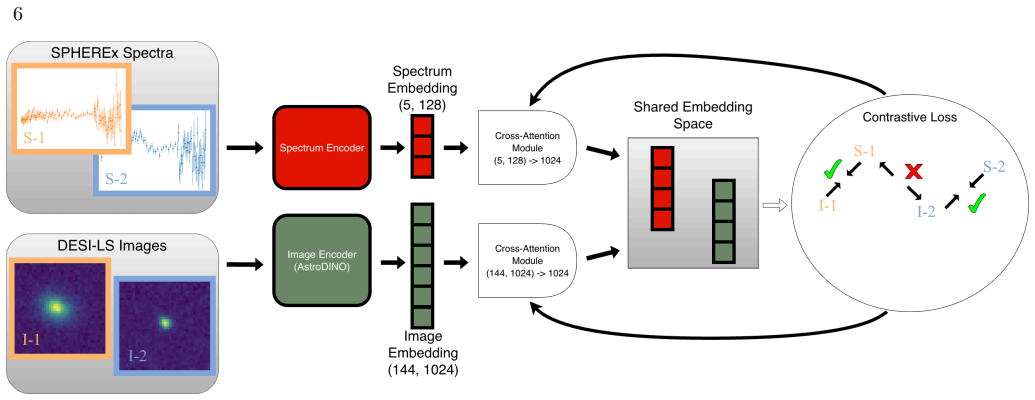
A CLIP-style contrastive alignment: an InfoNCE loss with cosine similarity pulls image and spectrum embeddings of the same source together and pushes different sources apart in a shared latent space. Images are encoded by a pre-trained transformer and spectra by a 1D convolutional autoencoder, with multi-head cross-attention projection heads generating 1024-dimensional embeddings; encoders are frozen, only the projection heads train. Downstream, XGBoost classifiers operate on these embeddings, and linear probes measure how accessible redshift and spectral fluxes are. The alignment is what reorganizes the embedding geometry; the paper's key evidence is that this reorganization, not new inform
Load-bearing premise
The load-bearing premise is that the mock SPHEREx spectra and injected stars are as hard to separate as real data; if real spectra, source blending, PSF errors, or noise inhomogeneity make stars and galaxies less separable, the measured gains and the sub-percent contamination forecast will not hold.
What would settle it
Run the same aligned-image classifier on real SPHEREx spectra and DESI-LS cutouts with labels from Gaia and Euclid across 18<z_AB<22.5 and measure stellar purity at p=0.5; if it falls from the predicted ~0.93 toward the unaligned ~0.76, or if the median footprint contamination at p>0.7 exceeds 1%, the paper's forecast is refuted.
If this is right
- A DESI-LS image-only classifier, after alignment, reaches stellar purity 0.931 and galaxy completeness 0.961 on the z<22.5 mock sample, making imaging a much stronger star–galaxy separator than raw spectra alone.
- Adopting p_gal>0.7 with a sigma_z/(1+z)<0.2 cut yields a predicted median stellar contamination of 0.4% over the SPHEREx extragalactic footprint, with 90% of tiles below 0.9%, meeting sub-percent requirements for sigma(f_NL)~O(1) analyses.
- Aligned embeddings degrade little when the classifier is simplified: a logistic regression stays within about 0.003 AUC of the full XGBoost model, implying contamination control will be less sensitive to classifier complexity and likely to systematic perturbations.
- Alignment disproportionately fixes the hardest subpopulations: galaxies at z~0.7–0.9 with 1.4<r-z<2.2, which overlap the stellar locus, are exactly the ones whose image embeddings become linearly separable.
- Completeness losses from aggressive purity cuts concentrate at low redshift, where SPHEREx samples remain sample-variance limited, so the purity/completeness tradeoff is affordable for clustering analyses.
Where Pith is reading between the lines
- The same contrastive recipe could be applied to other imaging surveys paired with any spectrophotometric catalog; the gain should be largest wherever morphology and broadband colors alone are degenerate, since alignment imports spectral discriminants into the image embedding.
- Because alignment mostly exposes information already in the imaging, it is a cheaper alternative to adding new bands: no new observations are needed, only a paired spectral catalog at train time. A testable prediction is that gains shrink as survey depth or PSF quality degrades.
- The mechanism suggests a broader design principle: contrastive alignment can act as a prior that linearizes classification boundaries, so for any high-dimensional astronomical classification task with paired modalities, aligned embeddings should outperform raw embeddings under simple models.
- A direct test would be to check whether the 1.6-micron H- opacity minimum, fixed in observed wavelength for stars and redshifted for galaxies, is what the aligned image embeddings encode; if so, galaxy sub-samples selected by aligned-image probability should have redshift distributions matching those implied by that feature.
Editorial analysis
A structured set of objections, weighed in public.
Referee Report
Summary. The paper presents a CLIP-style contrastive alignment between DESI Legacy Survey images and synthetic SPHEREx spectrophotometry, with the goal of improving star–galaxy separation for the SPHEREx galaxy survey. Using galaxy spectra generated from COSMOS template fits and synthetic stars injected into DESI-LS cutouts, the authors find that aligned embeddings outperform unaligned ones, especially for image-based classification: Table 1 reports galaxy purity 0.9908 and galaxy completeness 0.9614 for aligned image embeddings versus 0.9810 and 0.8349 unaligned. The paper also shows that aligned embeddings are more linearly separable (Section 4.2.3), and it uses photo-z precision cuts to forecast stellar contamination over the full SPHEREx footprint, concluding that sub-percent contamination is achievable with p_gal>0.7 (Section 5.3). The evaluation is entirely synthetic, with caveats acknowledged in Section 5.4.
Significance. If the results transfer to real data, the paper would provide a practical method for improving star–galaxy separation in SPHEREx and Rubin LSST, directly relevant to f_NL science goals. The study is carefully designed: it uses a clean paired image–spectrum construction, compares aligned versus unaligned embeddings under controlled conditions, and includes classifier ablation tests that strengthen the interpretation that alignment restructures the embedding space. The use of publicly available synthetic spectral data (Feder et al. 2023 on Zenodo) and standard open-source tools supports reproducibility. However, the central quantitative claims—the gain in image-based classification and the sub-percent contamination forecast—rest on the realism of the mocks and on the photo-z selection; both need stronger support before the abstract-level claims can be accepted.
major comments (4)
- [§5.3, Fig. 12] The sub-percent contamination forecast is derived entirely from synthetic data: galaxies are template SEDs from Feder et al. (2023) and stars are injected at blank-sky positions with a minimum separation of 1.5″ (Section 2.2.3). The caveats in Section 5.4 are qualitative; no quantitative estimate is given for how source blending, spatial noise inhomogeneity, or PSF errors would change η_star. Since the abstract states that contamination 'can be controlled at the sub-percent level across most of the extragalactic sky,' the authors should either validate with real SPHEREx/DESI-LS data (e.g., using Gaia/Euclid cross-checks) or provide a mock-degradation study that quantifies the impact of these effects. Without this, the abstract overstates the strength of the forecast.
- [§5.1, Fig. 10] The photo-z precision cut σ_z/(1+z)<0.2 is computed with a template-fitting code whose model grid matches the same template grid used to generate the synthetic galaxy SEDs. This creates a circularity: stars whose spectra resemble template galaxies at moderate redshift may be assigned large photo-z errors and removed preferentially, which is the main lever that suppresses contamination in the forecast. Please test sensitivity to an independent photo-z method (e.g., a different template set, a neural photo-z estimator, or real stellar SEDs) and report how the contamination fractions in §5.3 change. This is a load-bearing point because a factor-of-two change in the high-redshift stellar tail would materially alter the conclusion.
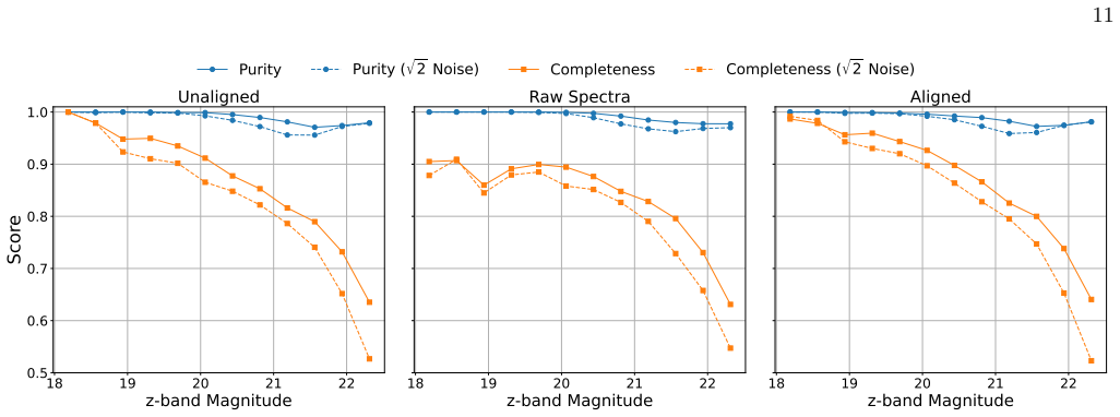
- [Table 1, §4.2.2] The classification metrics are reported without error bars, even though the 5-fold cross-validation procedure yields a distribution. The image-based improvement claims rely on differences of ~17 percentage points in stellar purity and ~13 percentage points in galaxy completeness; reporting fold-to-fold scatter or bootstrap uncertainties is necessary to confirm that the improvement is not driven by a particular split. The same applies to the AUC values in Figure 8 and the completeness/purity curves in Figures 6 and 11.
- [§4.2.1 and §5.3] The stellar-density correction is hand-calibrated to a ~50% overprediction near COSMOS and then extrapolated to the full sky using Gaia star counts. This correction is applied as a fixed factor, and its uncertainty is not propagated into the contamination forecast. Moreover, as the authors note in Section 5.4, Gaia may not trace the same stellar populations that leak into galaxy samples. Please provide a sensitivity analysis—e.g., varying the correction factor by ±50%—and show how the median and the 90/99th-percentile contamination fractions in Figure 12 change.
minor comments (5)
- [§4.2.4, Table 2] The subsample R² values are computed on the set of sources that are misclassified before alignment and correctly classified after. The sample size and the restricted range of this subset should be stated; R² on small, selected subsets can be noisy and should be interpreted with caution.
- [§5.3] The sentence 'η_star has a median of 1.3%, with 90% of the footprint having η_star<2.2% for 90% of HEALPix tiles and <3.6% for 99% of tiles' is confusing. Please rephrase, e.g., 'the median contamination fraction is 1.3%; 90% of the footprint has η_star<2.2% and 99% has η_star<3.6%.'
- [§3.2] The text describes the 102-channel SPHEREx data as 'photometry' in the sentence 'mapping the 102-channel photometry to a 6-dimensional latent space.' These are low-resolution spectral channels, not broadband photometry; please adjust the terminology for clarity.
- [Figure 3] The caption contains a typo: 'In the top bottom' should read 'In the bottom row.'
- [§2.2.3] The definition of the blank-sky injection separation θ_min=1.5″ is clear, but the paper does not state how many injected stars were rejected for lack of valid blank-sky positions. A sentence on the success rate would help assess potential selection biases.
Circularity Check
No significant circularity: the central classification and contamination results are measured on held-out synthetic data and do not reduce to fitted inputs or same-author self-citations.
full rationale
The derivation chain is self-contained and its main quantitative claims are not equivalent to the inputs by construction. The contrastive alignment (Eq. 1) is trained on image–spectrum pairs without using star/galaxy labels; labels enter only at the XGBoost stage, and Table 1 metrics are computed on held-out validation folds (5-fold CV, §4.2.2). The image-based classification gains therefore measure genuine generalization within the mock distribution, not the training loss itself. The contamination forecast (§5.3) rescales measured per-object false-positive rates using Gaia stellar-density maps; the only calibrated parameter is the ~50% stellar-density correction (§4.2.1), which the paper explicitly labels approximate ('We caution that this correction is approximate and defer a full comparison of simulations and data to future work') and which changes normalization, not the mechanism. The one same-author citation, Feder et al. (2023), supplies the synthetic galaxy SEDs; it is public on Zenodo, its template and emission-line assumptions are stated, and the stellar SEDs come from an independent BaSeL/pystellib model, so the classification is not forced by that citation. The photo-z step (§5.1) uses the Stickley et al. code with a Feder et al. grid, but this is a standard mock-reality test: the stellar spectra are not drawn from that galaxy grid, and the paper itself calls the high-redshift stellar solutions 'fictitious,' showing they are an output, not an input. The paper's own §5.4 and Conclusion explicitly identify the real-data validation gap ('Validating and extending these methods will require testing on real SPHEREx spectra and imaging'), which is an external-validity limitation, not circularity. No fitted parameter is renamed as a prediction, and no 'uniqueness' theorem is imported from the authors' prior work.
Axiom & Free-Parameter Ledger
free parameters (6)
- mock stellar density correction factor =
~1.5 (mocks overpredict Gaia star counts by ~50% near COSMOS)
- uniform E(B-V)=0.02 reddening for synthetic stars =
0.02
- blank-sky injection minimum separation theta_min=1.5 arcsec =
1.5 arcsec
- CLIP temperature tau =
15.0
- autoencoder bottleneck dimension =
6 (12 tested)
- XGBoost default hyperparameters =
200 trees, max depth 6
axioms (6)
- domain assumption SPHEREx synthetic spectra from Feder et al. (2023) realistically emulate real SPHEREx spectrophotometry, including photometric noise.
- domain assumption pystellib/BaSeL synthetic stellar SEDs, Galaxia spatial distribution, and PSF injection accurately represent the real stellar population seen by DESI-LS and SPHEREx.
- domain assumption The AstroDINO image encoder, pretrained on DESI-LS galaxies, retains enough information for star-galaxy separation after alignment.
- domain assumption The template-fitting photo-z code of Stickley et al. (2016) produces usable p(z) distributions for both stars and galaxies when applied to synthetic SPHEREx spectra.
- standard math The InfoNCE/CLIP contrastive objective is a valid proxy for maximizing mutual information between paired image and spectrum embeddings.
- domain assumption COSMOS 2020 templates plus the semi-empirical emission-line model of Feder et al. (2023) cover the true diversity of galaxies at z<2 in the SPHEREx sample.
read the original abstract
Stellar contamination is a critical systematic for increasingly precise large-scale structure analyses from ongoing and next-generation surveys. Experiments targeting constraints on local primordial non-Gaussianity with $\sigma(f_{\rm NL}^{\rm loc}) \sim \mathcal{O}(1)$ demand sub-percent stellar contamination rates to avoid misidentifying spurious large-scale power induced by Galactic structure as true cosmological signal. In this work, we explore the use of multimodal models for star--galaxy separation, harnessing the information from both optical broad-band imaging data and SPHEREx near-infrared low-resolution spectrophotometry. The two modalities are integrated using contrastive learning, which projects image- and spectrum-based embeddings into a shared latent space. We find that classifiers trained on these transformed representations outperform those trained on the original embeddings and show less performance degradation when simpler classifiers are used. These results suggest that multimodal alignment organizes the embedding space along dimensions that are better suited to source classification. The improvement is particularly strong for image-based classification, which we connect to increased predictability of highly-discriminative infrared spectral features from the transformed image embeddings. Applying redshift error-based selections and extrapolating to the full SPHEREx footprint, we demonstrate that stellar contamination can be controlled at the sub-percent level across most of the extragalactic sky, with completeness tradeoffs largely confined to low redshift. Our work highlights the utility of multimodal methods for modern galaxy surveys such as SPHEREx and $\textit{Rubin}$ LSST.
Figures





Reference graph
Works this paper leans on
-
[1]
Akeson, R., Dubois-Felsmann, G. P., Crill, B. P., et al. 2025, arXiv e-prints, arXiv:2511.15823, doi: 10.48550/arXiv.2511.15823 Astropy Collaboration, Robitaille, T. P., Tollerud, E. J., et al. 2013, A&A, 558, A33, doi: 10.1051/0004-6361/201322068
-
[2]
2014, doi: 10.48550/arXiv.1403.5237
Benitez, N., Dupke, R., Moles, M., et al. 2014, doi: 10.48550/arXiv.1403.5237
-
[3]
2011, in Astronomical Society of the Pacific Conference Series, Vol
Bertin, E. 2011, in Astronomical Society of the Pacific Conference Series, Vol. 442, Astronomical Data Analysis Software and Systems XX, ed. I. N. Evans, A. Accomazzi, D. J. Mink, & A. H. Rots, 435
2011
-
[4]
Bock, J. J., Aboobaker, A. M., Adamo, J., et al. 2025, arXiv e-prints, arXiv:2511.02985, doi: 10.48550/arXiv.2511.02985 21
-
[5]
2016, arXiv e-prints, arXiv:1603.02754, doi: 10.48550/arXiv.1603.02754
Chen, T., & Guestrin, C. 2016, arXiv e-prints, arXiv:1603.02754, doi: 10.48550/arXiv.1603.02754
-
[6]
Clarke, A. O., Scaife, A. M. M., Greenhalgh, R., & Griguta, V. 2020, A&A, 639, A84, doi: 10.1051/0004-6361/201936770 de Jong, J. T. A., Verdoes Kleijn, G. A., Kuijken, K. H., &
-
[7]
Valentijn, E. A. 2013, Experimental Astronomy, 35, 25, doi: 10.1007/s10686-012-9306-1 DESI Collaboration, Aghamousa, A., Aguilar, J., et al. 2016, arXiv e-prints, arXiv:1611.00036, doi: 10.48550/arXiv.1611.00036 DESI Legacy Surveys. 2023, Galactic Extinction Coefficients, https://www.legacysurvey.org/dr10/ catalogs/#galactic-extinction-coefficients
-
[8]
2019, The Astronomical Journal, 157, 168, doi: 10.3847/1538-3881/ab089d
Dey, A., et al. 2019, The Astronomical Journal, 157, 168, doi: 10.3847/1538-3881/ab089d
-
[9]
Feder, R. M., Masters, D. C., Lee, B., et al. 2023, arXiv e-prints, arXiv:2312.04636, doi: 10.48550/arXiv.2312.04636
-
[10]
Fitzpatrick, E. L. 1999, PASP, 111, 63 Gagn´ e, J., Faherty, J. K., Ruiz Diaz, A., et al. 2026, arXiv e-prints, arXiv:2604.22012, doi: 10.48550/arXiv.2604.22012 Gaia Collaboration, Vallenari, A., Brown, A. G. A., et al. 2023, A&A, 674, A1, doi: 10.1051/0004-6361/202243940
-
[11]
Girardi, L., Groenewegen, M. A. T., Hatziminaoglou, E., & da Costa, L. 2005, A&A, 436, 895, doi: 10.1051/0004-6361:20042352 Gopalakrishnan Nair, N., Gedara Chaminda Bandara, W., & Patel, V. M. 2022, arXiv e-prints, arXiv:2206.05039, doi: 10.48550/arXiv.2206.05039
work page internal anchor Pith review Pith/arXiv arXiv doi:10.48550/arxiv.2206.05039 2005
-
[12]
Harris, C. R., Millman, K. J., van der Walt, S. J., et al. 2020, Nature, 585, 357, doi: 10.1038/s41586-020-2649-2
-
[13]
Huai, Z., Bock, J. J., Cheng, Y.-T., et al. 2025, arXiv e-prints, arXiv:2510.01410, doi: 10.48550/arXiv.2510.01410
-
[14]
Hunter, J. D. 2007, Computing in Science & Engineering, 9, 90, doi: 10.1109/MCSE.2007.55 Ivezi´ c,ˇZ., Kahn, S. M., Tyson, J. A., et al. 2019, ApJ, 873, 111, doi: 10.3847/1538-4357/ab042c
-
[15]
P., Vieira dos Santos, G., Marra, V., et al
Jeakel, A. P., Vieira dos Santos, G., Marra, V., et al. 2025, arXiv e-prints, arXiv:2511.20524. https://arxiv.org/abs/2511.20524
arXiv 2025
-
[16]
W., & Mykytyn, D
Lang, D., Hogg, D. W., & Mykytyn, D. 2016, The Tractor: Probabilistic astronomical source detection and measurement, Astrophysics Source Code Library, record ascl:1604.008. http://ascl.net/1604.008
2016
-
[17]
1997, A&AS, 125, 229, doi: 10.1051/aas:1997373
Lejeune, T., Cuisinier, F., & Buser, R. 1997, A&AS, 125, 229, doi: 10.1051/aas:1997373
-
[18]
2019, arXiv preprint arXiv:1711.05101
Loshchilov, I., & Hutter, F. 2019, arXiv preprint arXiv:1711.05101
Pith/arXiv arXiv 2019
-
[19]
2020, in Proceedings of Machine Learning Research, Vol
McAllester, D., & Stratos, K. 2020, in Proceedings of Machine Learning Research, Vol. 108, Proceedings of the Twenty Third International Conference on Artificial Intelligence and Statistics, ed. S. Chiappa & R. Calandra (PMLR), 875–884. https://proceedings.mlr.press/v108/mcallester20a.html
2020
-
[20]
2018, arXiv preprint arXiv:1802.03426
McInnes, L., Healy, J., & Melville, J. 2018, arXiv preprint arXiv:1802.03426
Pith/arXiv arXiv 2018
-
[21]
2024, MNRAS, 531, 4990, doi: 10.1093/mnras/stae1450
Parker, L., Lanusse, F., Golkar, S., et al. 2024, MNRAS, 531, 4990, doi: 10.1093/mnras/stae1450
-
[22]
2025, arXiv e-prints, doi: 10.48550/arXiv.2510.17960
Parker, L., Lanusse, F., Shen, J., et al. 2025, arXiv e-prints, doi: 10.48550/arXiv.2510.17960
-
[23]
2019, in Advances in Neural Information Processing Systems 32 (Curran Associates, Inc.), 8024–8035
Paszke, A., Gross, S., et al. 2019, in Advances in Neural Information Processing Systems 32 (Curran Associates, Inc.), 8024–8035. http://nips.cc
2019
-
[24]
Radford, A., Kim, J. W., Hallacy, C., et al. 2021, arXiv e-prints, arXiv:2103.00020, doi: 10.48550/arXiv.2103.00020
-
[25]
2026, arXiv e-prints, arXiv:2607.00543
Rustamkulov, Z., Kirkpatrick, J., Akeson, R., et al. 2026, arXiv e-prints, arXiv:2607.00543. https://arxiv.org/abs/2607.00543
Pith/arXiv arXiv 2026
-
[26]
2002, The Astronomical Journal, 124, 3050, doi: 10.1086/344682
Sawicki, M. 2002, The Astronomical Journal, 124, 3050, doi: 10.1086/344682
doi:10.1086/344682 2002
-
[27]
2007, The Astrophysical Journal Supplement Series, 172, 1, doi: 10.1086/516585
Scoville, N., Aussel, H., Brusa, M., et al. 2007, The Astrophysical Journal Supplement Series, 172, 1, doi: 10.1086/516585
doi:10.1086/516585 2007
-
[28]
2011, ApJ, 730, 3, doi: 10.1088/0004-637X/730/1/3
Binney, J. 2011, ApJ, 730, 3, doi: 10.1088/0004-637X/730/1/3
-
[29]
R., Capak, P., Masters, D., et al
Stickley, N. R., Capak, P., Masters, D., et al. 2016, arXiv e-prints, arXiv:1606.06374, doi: 10.48550/arXiv.1606.06374 The Dark Energy Survey Collaboration. 2005, arXiv e-prints, astro, doi: 10.48550/arXiv.astro-ph/0510346 The Multimodal Universe Collaboration, Audenaert, J.,
-
[30]
Bowles, M., et al. 2024, arXiv e-prints, arXiv:2412.02527, doi: 10.48550/arXiv.2412.02527 van den Oord, A., Li, Y., & Vinyals, O. 2018, CoRR, abs/1807.03748. https://arxiv.org/abs/1807.03748
-
[31]
Virtanen, P., Gommers, R., Oliphant, T. E., et al. 2020, Nature Methods, 17, 261, doi: 10.1038/s41592-019-0686-2
-
[32]
Weaver, J. R., Kauffmann, O. B., Ilbert, O., et al. 2022, ApJS, 258, 11, doi: 10.3847/1538-4365/ac3078
-
[33]
2021, MNRAS, 503, 5061, doi: 10.1093/mnras/stab709
Weaverdyck, N., & Huterer, D. 2021, MNRAS, 503, 5061, doi: 10.1093/mnras/stab709
-
[34]
Wen, R. Y., Gebhardt, H. S. G., Heinrich, C., & Dor´ e, O. 2025, PhRvD, 112, 063518, doi: 10.1103/hqc3-tbxc
-
[35]
Yang, Y. et al. 2025, in prep. 22
2025
-
[36]
2026, ApJ, 998, 189, doi: 10.3847/1538-4357/ae2c7e
Zhao, X., Huang, Y., Xue, G., et al. 2026, ApJ, 998, 189, doi: 10.3847/1538-4357/ae2c7e
-
[37]
Zhou, R., Dey, B., Newman, J. A., et al. 2023, AJ, 165, 58, doi: 10.3847/1538-3881/aca5fb
discussion (0)
Sign in with ORCID, Apple, or X to comment. Anyone can read and Pith papers without signing in.