REVIEW 7 minor 71 references
Spectro-polarimetric radio imaging with SKA can map coronal magnetic fields that optical methods and extrapolations cannot reach.
Reviewed by Pith at T0; open to challenge. T0 means a machine referee read the full paper against a public rubric. the ladder, T0–T4 →
T0 review · grok-4.5
2026-07-12 01:07 UTC pith:P4KV23DF
load-bearing objection Solid, well-referenced SKA science-case chapter that maps established radio coronal-B diagnostics onto SKA-Low/Mid capabilities; no new physics, but useful and referee-ready as a review.
Coronal Magnetography using Spectropolarimetry with SKA Telescopes
The pith
A machine-rendered reading of the paper's core claim, the machinery that carries it, and where it could break.
Core claim
The paper’s central claim is that high-fidelity spectro-polarimetric imaging across SKA’s 0.05–15 GHz band will turn free-free circular polarization, gyro-resonance layer heights, gyrosynchrotron spectra and the polarization of radio bursts into quantitative, multi-height coronal magnetograms that optical techniques and photospheric extrapolations cannot supply.
What carries the argument
The mapping of magneto-ionic modes (x-mode versus o-mode) and their absorption, emission and mode-coupling signatures onto measurable Stokes-V (and, for some bursts, linear) polarization; each emission process thereby becomes a direct or semi-direct probe of local B.
Load-bearing premise
That residual instrumental leakage, ionospheric Faraday rotation and direction-dependent beam errors at low frequencies can be calibrated well enough to recover the few-percent circular-polarization signals on which free-free and harmonic plasma diagnostics rest.
What would settle it
A full-Stokes solar imaging campaign with SKA (or a pathfinder at comparable fidelity) that either recovers or fails to recover the expected free-free circular polarization of order 1–10 % above a well-observed active region or streamer whose field strength is independently constrained by multi-wavelength density and temperature diagnostics.
Editorial analysis
A structured set of objections, weighed in public.
Referee Report
Summary. This chapter reviews remote-sensing techniques for measuring solar coronal magnetic fields via radio spectro-polarimetry and argues that SKA-Low and SKA-Mid will enable transformative multi-height magnetography. It covers free-free emission (weak circular polarization giving B_LoS via the standard QL approximation), gyroresonance (iso-Gauss layers above active regions and bright points), gyrosynchrotron (flaring loops and CMEs), plasma emission (type II/III/IV bursts, band-splitting, and harmonic polarization), fibre/zebra fine structures, and propagation effects (QT mode coupling and polarization inversion). Established formulae (e.g., free-free V_frac, gyroresonance optical depth, Rankine–Hugoniot compression, Cohen Q) are correctly cited and illustrated with precursor results from MWA, MeerKAT, EOVSA, NoRH and RATAN-600. Section 4 maps these diagnostics onto SKA AA* capabilities (bandwidth, sensitivity, resolution, subarrays) and coordinated multi-wavelength observations.
Significance. Coronal magnetography remains a central unsolved problem for solar physics and space weather. The manuscript provides a clear, multi-mechanism synthesis that correctly situates radio diagnostics relative to optical/EUV Zeeman/Hanle methods and photospheric extrapolations. Its value lies in the systematic linkage of well-established emission physics to concrete SKA observing modes and in the explicit incorporation of recent precursor advances (MWA leakage pipelines, MeerKAT bright-point imaging, EOVSA GS spectral fitting). If the calibration path outlined in §4.1 succeeds, the chapter supplies a practical roadmap for routine 2-D/3-D coronal field constraints across quiet Sun, active regions and eruptive events.
minor comments (7)
- Throughout: several compound words are missing spaces or hyphens (e.g., “spaceweathertothemuchweakernanoflares”, “high-fidelitypolarimetric”, “widebandobservations”). A global copy-edit pass is needed.
- Eq. (11) and surrounding text: the numerical prefactor 5400 assumes cgs units and the QL approximation; a one-sentence reminder of the validity regime (ν_B/ν ≪ 1, independent T) would help non-specialist readers.
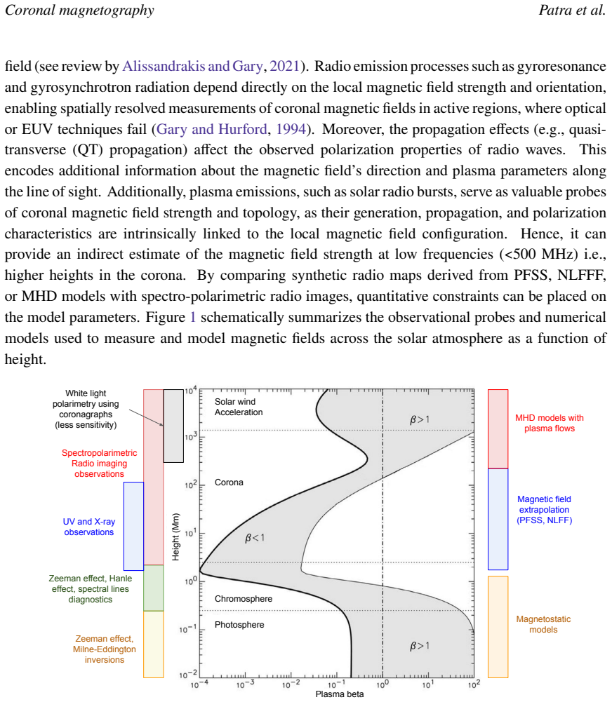
- Figure 1 caption and body: the original Gary (2001) plasma-β schematic is useful, but the overlaid radio-probe labels would benefit from a short legend distinguishing free-free, gyroresonance and plasma-emission height ranges.
- Section 3.4.2 (type II): the two competing interpretations of band-splitting (upstream/downstream vs. different shock locations) are both cited; a brief statement of which assumption is adopted for the B estimates that follow would reduce ambiguity.
- Section 4.1: the discussion of polconversion/polrotation and ionospheric Faraday rotation is appropriately cautious; adding a quantitative target (e.g., residual leakage ≲ 0.1–1 % for free-free V) would make the calibration requirement more concrete.
- Table 1: heights and B values are useful; adding the assumed density model or scale length used in each study would improve reproducibility.
- References: a few arXiv-only or “in preparation” entries (e.g., Oberoi et al. 2026, Mondal et al. 2026) should be updated or flagged as companion AASKAII chapters if they remain unpublished at acceptance.
Circularity Check
No circularity: prospective review applying established radio diagnostics to SKA capabilities; no fitted-as-prediction or self-definitional steps.
full rationale
This is a science-case chapter for Advancing Astrophysics with the SKA – II, not a primary derivation paper. Section 3 reviews free-free (Eqs. 1–11 from Zlotnik/Dulk/Fleishman), gyro-resonance (Eq. 12 from White & Kundu), gyrosynchrotron (Ramaty/Dulk), plasma emission (Eq. 14 from Melrose et al.), and mode-coupling (Eqs. 18–22 from Cohen/Zheleznyakov) diagnostics, all taken from the external literature and applied forward. Section 4 then maps those established techniques onto SKA-Low/Mid bandwidth, sensitivity, and polarimetric imaging, citing the authors’ own precursor pipelines (MWA leakage calibration, MeerKAT bright-point imaging) only as demonstrated technical progress, not as uniqueness theorems or load-bearing uniqueness claims that force the central result. No parameter is fitted to data and then re-labeled a prediction; no equation is defined in terms of the quantity it purports to derive; no ansatz is smuggled in via self-citation. The residual calibration risk for weak Stokes-V is openly flagged by the authors themselves (§4.1) rather than hidden. The derivation chain is therefore self-contained against external benchmarks and exhibits no circular reduction.
Axiom & Free-Parameter Ledger
axioms (4)
- domain assumption Cold-plasma magneto-ionic theory (QL/QT approximations, mode-coupling parameter Q) correctly describes radio-wave propagation in the solar corona.
- domain assumption Gyroresonance optical depth is significant only for the 2nd and 3rd harmonics under typical coronal temperatures and densities.
- domain assumption Type-II band splitting arises from upstream/downstream shock regions (Rankine–Hugoniot), allowing Alfvén-speed and B estimates.
- domain assumption SKA-Low (307 stations) and SKA-Mid (144 dishes) AA* configurations will deliver the stated instantaneous bandwidths, baselines and imaging dynamic range.
read the original abstract
The solar coronal magnetic field drives nearly every aspect of solar phenomena and activity -- from flares, coronal mass ejections, and solar wind that governs space weather to the much weaker nanoflares. These magnetic fields are routinely measured at the visible surface of the Sun, the photosphere. However, detailed and direct measurements of the magnetic fields in the solar atmosphere, particularly in the coronal layer, have remained rather limited. Mostly, these are estimated from vector magnetic field measurements at photospheric heights through different extrapolation models. In the case of the corona, these extrapolations lack observational constraints from the corona, especially during periods of intense activity when magnetic structures evolve rapidly. Measurements of coronal magnetic fields from observations, therefore, remain one of the most crucial and unresolved challenges in solar and space-weather research. Radio observations of the Sun hold considerable potential in this regard. Observations of diverse emission mechanisms, ranging from plasma emissions at lower frequencies to thermal Bremsstrahlung and gyro-resonance at higher frequencies, provide multiple avenues to probe the coronal magnetic fields, unique at radio wavelengths. SKAO, with its broad frequency coverage (0.05 to 15 GHz), will allow us to probe wide range of coronal layers through unprecedented high-fidelity polarimetric imaging at high temporal, spectral, and spatial resolutions. This chapter details how the coronal magnetic field measurements can be achieved through spectro-polarimetric imaging of the Sun with the SKAO.
Figures


Reference graph
Works this paper leans on
-
[1]
doi: 10.1007/BF00146972. C. Alissandrakis, M. Kundu, and P. Lantos.Astronomy and Astrophysics, vol. 82, no. 1-2, Feb. 1980, p. 30-40., 82:30–40,
-
[2]
H.Aurass,G.Rausche,G.Mann,andA.Hofmann.Astronomy&Astrophysics,435(3):1137–1148,
doi: 10.1051/0004-6361/202141672. H.Aurass,G.Rausche,G.Mann,andA.Hofmann.Astronomy&Astrophysics,435(3):1137–1148,
-
[3]
doi: 10.1088/0004-637X/782/1/43. R. Bandiera.Astronomy and Astrophysics, vol. 112, no. 1, Aug. 1982, p. 52-60., 112:52–60,
-
[4]
doi: 10.1086/323421. A. O. Benz and G. Mann.Astronomy and Astrophysics, v. 333, p. 1034-1042 (1998), 333:1034– 1042,
doi:10.1086/323421 1998
-
[5]
T. E. Bernold and R. A. Treumann.Astrophysical Journal, Part 1, vol. 264, Jan. 15, 1983, p. 677-688. Research supported by the Swiss National Science Foundation and Swiss Society for Astronomy and Astrophysics., 264:677–688,
1983
-
[6]
doi: 10.1051/0004-6361/202244456. V. Bogod and G. Gelfreikh.Solar Physics, 67(1):29–46,
-
[7]
URLhttps: //doi.org/10.1051/0004-6361/202346788
doi: 10.1051/0004-6361/202346788. URLhttps: //doi.org/10.1051/0004-6361/202346788. J. W. Brosius et al.The Astrophysical Journal, 574(1):453,
-
[8]
doi: 10.1051/0004-6361/201731368. B. Chen et al.Nature Astronomy, 4(12):1140–1147,
-
[9]
doi: 10.1051/0004-6361/201015578. M. H. Cohen.Astrophysical Journal, vol. 131, p. 664, 131:664,
-
[10]
doi: 10.3847/1538-3881/acabc3. C. DeForest et al.arXiv e-prints, page arXiv:2509.15131,
-
[11]
doi: 10.48550/arXiv.2509.15131. S. Dey, D. Kansabanik, D. Oberoi, and S. Mondal. ApJ, 988(2):L73, Aug
-
[12]
doi: 10.3847/ 2041-8213/adef0e. Dey, S. et al.Astronomy & Astrophysics, 704:A75,
2041
-
[13]
URLhttps://doi.org/10.1051/0004-6361/202556857
doi: 10.1051/0004-6361/202556857. URLhttps://doi.org/10.1051/0004-6361/202556857. C. Downs et al.Science, page eadq0872,
-
[14]
doi: 10.1088/2041-8205/793/2/L39. G. A. Dulk. ARA&A, 23:169–224, Jan
-
[15]
25 Coronal magnetography Patra et al
doi: 10.1146/annurev.aa.23.090185.001125. 25 Coronal magnetography Patra et al. G. A. Dulk and S. Suzuki. A&A, 88(1-2):203–217, Aug
-
[16]
doi: 10.1007/BF00153154. G. D. Fleishman and V. F. Melnikov. ApJ, 587(2):823–835, Apr
-
[17]
doi: 10.1086/368252. G. D. Fleishman et al.Science, 367(6475):278–280,
-
[18]
doi: 10.3847/1538-4357/aad0ef. D. E. Gary et al.The Astrophysical Journal, 863(1):83,
-
[19]
S.E.Gibsonetal.FrontiersinAstronomyandSpaceSciences,Volume3-2016,2016. ISSN2296- 987X. doi: 10.3389/fspas.2016.00008. URLhttps://www.frontiersin.org/journals/ astronomy-and-space-sciences/articles/10.3389/fspas.2016.00008. V. L. Ginzburg, W. L. Sadowski, D. Gallik, and S. C. Brown.Physics Today, 15(10):70–73,
-
[20]
doi: 10.1088/0004-637X/744/1/72. G. Hallinan et al. InAmerican Astronomical Society Meeting Abstracts #241, volume 241 of American Astronomical Society Meeting Abstracts, page 451.09, Jan
-
[21]
doi: 10.1088/0004-637X/795/1/14. K. Hariharan, R. Ramesh, and C. Kathiravan. Sol. Phys., 290(9):2479–2489, Sept
-
[22]
K.Hariharan,R.Ramesh,C.Kathiravan,andT.J.Wang
doi: 10.1007/s11207-015-0761-5. K.Hariharan,R.Ramesh,C.Kathiravan,andT.J.Wang. Sol.Phys.,291(5):1405–1416,May2016. doi: 10.1007/s11207-016-0918-x. B. C. Hicks et al. PASP, 124(920):1090, Oct
-
[23]
doi: 10.1086/668121. K. Iwai et al.Earth, Planets and Space, 66(1):149,
-
[24]
26 Coronal magnetography Patra et al
doi: 10.1017/S1323358000011383. 26 Coronal magnetography Patra et al. T. Kakinuma and G. Swarup.Astrophysical Journal, vol. 136, p. 975, 136:975,
-
[28]
doi: 10.3389/fspas.2025.1666743
ISSN 2296-987X. doi: 10.3389/fspas.2025.1666743. URL https://www.frontiersin.org/journals/astronomy-and-space-sciences/ articles/10.3389/fspas.2025.1666743. D. Kansabanik et al. ApJS, 278(1):26, May
-
[29]
doi: 10.3847/1538-4365/adc443. K. G. Klein et al.Space Science Reviews, 219(8):74,
-
[30]
doi: 10.1071/PH580201. A. Kouloumvakos et al. ApJ, 913(2):99, June
-
[31]
doi: 10.3847/1538-4357/abf435. H. A. Kramers.The London, Edinburgh, and Dublin Philosophical Magazine and Journal of Science, 46(275):836–871,
-
[32]
A. Kumari, R. Ramesh, C. Kathiravan, and N. Gopalswamy. ApJ, 843(1):10, July 2017a. doi: 10.3847/1538-4357/aa72e7. A. Kumari, R. Ramesh, C. Kathiravan, and T. J. Wang. Sol. Phys., 292(11):161, November 2017b. doi: 10.1007/s11207-017-1180-6. A. Kumari et al. ApJ, 881(1):24, August
-
[33]
doi: 10.3847/1538-4357/ab2adf. M. Kundu and C. Alissandrakis.Solar physics, 94(2):249–283,
-
[34]
doi: 10.1007/978-94-010-3587-3_21. M. R. Kundu.New York: Interscience Publication,
-
[35]
doi: 10.1007/BF00148288. A. Kuznetsov and E. Kontar.Solar Physics, 290(1):79–93,
-
[36]
doi: 10.1007/s11214-015-0219-y. K. Lang et al.Astrophysical Journal v. 419, p. 398, 419:398,
-
[37]
doi: 10.1007/s11207-011-9776-8. H. Lin, J. Kuhn, and R. Coulter.The Astrophysical Journal, 613(2):L177,
-
[38]
doi: 10.1016/j.jastp.2018.03.018. D. J. F. Maia et al. ApJ, 660(1):874–881, May
-
[39]
doi: 10.1086/508011. P. I. McCauley et al.Solar Physics, 294(8):106,
-
[40]
doi: 10.1086/160219. D. B. Melrose and W. N. Sy.Australian Journal of Physics, 25:387, Aug
-
[41]
doi: 10.1007/BF00156783. S. Mondal, D. Oberoi, and A. Mohan. ApJ, 895(2):L39, June 2020a. doi: 10.3847/2041-8213/ ab8817. S. Mondal, D. Oberoi, and A. Vourlidas. ApJ, 893(1):28, April 2020b. doi: 10.3847/1538-4357/ ab7fab. S. Mondal et al. InAdvancing Astrophysics with the SKA – II (AASKAII)
-
[42]
28 Coronal magnetography Patra et al
doi: 10.1051/0004-6361/201834510. 28 Coronal magnetography Patra et al. D. Müller et al. A&A, 642:A1, Oct
-
[43]
doi: 10.1051/0004-6361/202038467. J. Nagelis and B. Ryabov.Kinematics and Physics of Celestial Bodies, 8(6):28–32,
-
[44]
doi: 10.1093/pasj/37.1.163. H. Nakajima et al.IEEE Proceedings, 82(5):705–713, May
-
[45]
doi: 10.1109/5.284737. A. Nindos, S. White, M. Kundu, and D. Gary.The Astrophysical Journal, 533(2):1053,
-
[46]
doi: 10.1088/0004-637X/799/2/236. G. M. Nita et al.The Astrophysical Journal, 853(1):66,
-
[47]
M.PalombaandJ.-P.Luntama.44thCOSPARScientificAssembly.Held16-24July,44:3544,2022
arXiv search: Report number AASKAII/Oberoi01. M.PalombaandJ.-P.Luntama.44thCOSPARScientificAssembly.Held16-24July,44:3544,2022. R. A. Perley, C. J. Chandler, B. J. Butler, and J. M. Wrobel. ApJ, 739(1):L1, Sept
2022
-
[48]
doi: 10.1088/2041-8205/739/1/L1. B. Perri et al. ApJ, 936(1):19, aug
-
[49]
doi: 10.3847/1538-4357/ac7237. URLhttps://dx. doi.org/10.3847/1538-4357/ac7237. B. Perri et al. ApJ, 943(2):124, feb
-
[50]
URLhttps: //dx.doi.org/10.3847/1538-4357/ac9799
doi: 10.3847/1538-4357/ac9799. URLhttps: //dx.doi.org/10.3847/1538-4357/ac9799. N. Peterova and S. B. Akhmedov.Soviet Astronomy, Vol. 17, p. 768, 17:768,
-
[51]
doi: 10.1086/150235. R. Ramesh and C. Kathiravan. ApJ, 940(1):80, November
-
[52]
doi: 10.3847/1538-4357/ac9c65. R. Ramesh, C. Kathiravan, and C. V. Sastry.The Astrophysical Journal, 711(2):1029,
-
[53]
R.Ramesh,C.Kathiravan,andA.Kumari.ApJ,943(1):43,January2023.doi: 10.3847/1538-4357/ acaea5
doi: 10.3847/ 1538-4357/ac6f05. R.Ramesh,C.Kathiravan,andA.Kumari.ApJ,943(1):43,January2023.doi: 10.3847/1538-4357/ acaea5. N. E. Raouafi et al. Space Sci. Rev., 219(1):8, Feb
-
[54]
doi: 10.1007/s11214-023-00952-4. T. R. Rimmele et al.Solar Physics, 295(12):1–49,
-
[55]
doi: 10.1051/0004-6361/ 202037989. C. V. Sastry. ApJ, 697(2):1934–1939, June
-
[56]
doi: 10.1088/0004-637X/697/2/1934. R. J. Sault, J. P. Hamaker, and J. D. Bregman. A&AS, 117:149–159, May
-
[57]
URLhttps://doi.org/10.5281/zenodo.16950982. S. Segre and V. Zanza.The Astrophysical Journal, 554(1):408,
-
[58]
doi: 10.1017/pasa.2012.007. D. Tripathi et al.Proceedings of the International Astronomical Union, 18(S372):17–27,
-
[59]
doi: 10.1017/S1743921323001230. S. D. Tun and A. Vourlidas. ApJ, 766(2):130, April
-
[60]
doi: 10.1088/0004-637X/766/2/130. V. Tzatzakis, A. Nindos, and C. E. Alissandrakis. Sol. Phys., 253(1-2):79–94, Dec
-
[61]
doi: 10.1007/s11207-008-9263-z. B. van der Holst et al.The Astrophysical Journal, 782(2):81,
-
[62]
doi: 10.1051/0004-6361/201220873. V. Vasanth et al. ApJ, 830(1):L2, Oct
-
[63]
doi: 10.3847/2041-8205/830/1/L2. B. Vršnak, H. Aurass, J. Magdalenić, and N. Gopalswamy. A&A, 377:321–329, October
-
[64]
30 Coronal magnetography Patra et al
doi: 10.1051/0004-6361:20011067. 30 Coronal magnetography Patra et al. B.Vršnak,J.Magdalenić,H.Aurass,andG.Mann. A&A,396:673–682,Dec.2002. doi: 10.1051/ 0004-6361:20021413. M. Wang, C. C. Duan, R. X. Xie, and Y. H. Yan. Sol. Phys., 212(2):401–406, Feb
-
[65]
doi: 10.1023/A:1022939203483. S. White and M. Kundu.Solar Physics, 174(1):31–52,
-
[66]
J.WildandS.Smerd.AnnualReviewofAstronomyandAstrophysics,vol.10,p.159,10:159,1972. J. P. Wild. PASA, 1(2):38–39, Nov
1972
-
[67]
doi: 10.1017/S1323358000010407. Y. Yan et al.frontiers in Astronomy and Space Sciences, 8:584043,
-
[68]
InM.R.KunduandT.E.Gergely,editors,RadioPhysicsofthe Sun,volume86ofIAUSymposium,pages87–99,Jan.1980
V.V.ZhelezniakovandE.I.Zlotnik. InM.R.KunduandT.E.Gergely,editors,RadioPhysicsofthe Sun,volume86ofIAUSymposium,pages87–99,Jan.1980. doi: 10.1017/S0074180900036676. V. Zheleznyakov.Soviet Astronomy, Vol. 6, p. 3, 6:3,
-
[69]
V.ZheleznyakovandE.Y.Zlotnik.RadiophysicsandQuantumElectronics,20(9):997–1009,1977. A. N. Zhukov et al.arXiv e-prints, (arXiv:2509.00253),
Pith/arXiv arXiv 1977
-
[70]
doi: 10.48550/arXiv.2509.00253. I. Zimovets et al. A&A, 547:A6, Nov
-
[71]
doi: 10.1051/0004-6361/201219454. I. V. Zimovets and V. M. Sadykov.Advances in Space Research, 56(12):2811–2832, Dec
-
[72]
doi: 10.1016/j.asr.2015.01.041. E. I. Zlotnik. A&A, 101(2):250–258, Aug
-
[73]
doi: 10.1051/0004-6361/201732308. P. Zucca et al. A&A, 703:A271, Nov
-
[74]
doi: 10.1051/0004-6361/202554348. 31
discussion (0)
Sign in with ORCID, Apple, or X to comment. Anyone can read and Pith papers without signing in.