AMSFL: Adaptive Multi-Step Federated Learning via Gradient Difference-Based Error Modeling

Ganglou Xu

REVIEW 5 major objections 5 minor 11 references

AMSFL: Adaptive Multi-Step Federated Learning via Gradient Difference-Based Error Modeling

T0 review · 5 major / 5 minor · reviewed 2026-08-07 · deepseek-v4-flash

Challenge this review Re-run · record.json Download PDF Read on arXiv ↗

Pith's one-line read A first-order gradient-difference error model lets federated clients adapt their local step counts without Hessians.

desk verdict The adaptive step scheduler is a reasonable heuristic, but the paper's central optimality proof is wrong—the KKT solution contradicts the stated objective—so the theoretical claims don't stand. read the letter →

arxiv 2505.21695 v1 pith:PLPDLBU2 submitted 2025-05-27 cs.LG cs.DC

Ganglou Xu This is my paper

classification cs.LGcs.DC

keywords federatedlearningadaptivelocalstepsgradientdifferenceapproximationerrorpropagationnon-IIDdataconvergenceboundresource-constrainedtraining

verification ladder T0 review T1 audit T2 compute T3 formal

The pith

A machine-rendered reading of the paper's core claim, the machinery that carries it, and where it could break.

The reading

The paper proposes Gradient Difference Approximation (GDA), a first-order proxy for the second-order curvature effects that drive local update drift in federated learning, and embeds it in the Adaptive Multi-Step Federated Learning (AMSFL) framework. The central claim is that drift can be estimated from gradient differences alone, allowing each client to receive a tailored number of local SGD steps per round under a wall-clock budget. If correct, this gives better accuracy, faster convergence, and lower per-round latency than fixed-step baselines, without the cost of Hessian computation. Experiments on NSL-KDD report a global accuracy of 0.9023 and convergence to 89 percent accuracy in about 49 seconds.

What carries the argument

Gradient Difference Approximation (GDA), defined as replacing the Hessian-vector product in a Taylor expansion by the gradient difference between successive local models, with approximation error bounded by (L/2) times the squared norm of the update. GDA converts the otherwise expensive curvature term into a quantity obtainable from first-order information, and it feeds directly into the step-allocation theorem that assigns more local steps to clients with lower computational cost.

What would settle it

Measure the actual cumulative gradient-drift term on a non-strongly-convex objective and check whether the squared error of AMSFL remains under the claimed limsup bound; if the gap between the observed error and the bound widens or the error diverges, the theorem's applicability to the experimental setting does not hold.

Watch

Extended reading notes

Core claim

The paper establishes an error recursion for multi-step local updates under GDA, showing that after aggregation the global error satisfies a bound of the form limsup of the squared distance to optimum being no larger than a constant times a Drift term Delta_k that depends on step size, local step counts, and gradient deviation. It further shows that, when each client has a per-step cost, the optimal allocation of local steps under a total time budget is proportional to the inverse square root of that cost. The discovery is that the accumulated gradient-deviation term can be replaced by computable first-order gradient differences, making error-aware step control lightweight enough for resource-constrained clients.

Load-bearing premise

The residual-error theorem assumes the global objective is strongly convex, yet strong convexity is not listed among the paper's assumptions and does not hold for the deep network used in the experiments.

Editorial extensions

If this is right

Clients with cheaper per-step computation will be assigned more local steps, and more expensive clients fewer, while respecting a total time budget.
Adaptive multi-step training can be conducted round by round using only gradient differences, without Hessian-vector products or second-order solvers.
The residual error bound degrades with larger step sizes and more local updates, which can guide practitioners toward safer settings of these hyperparameters.
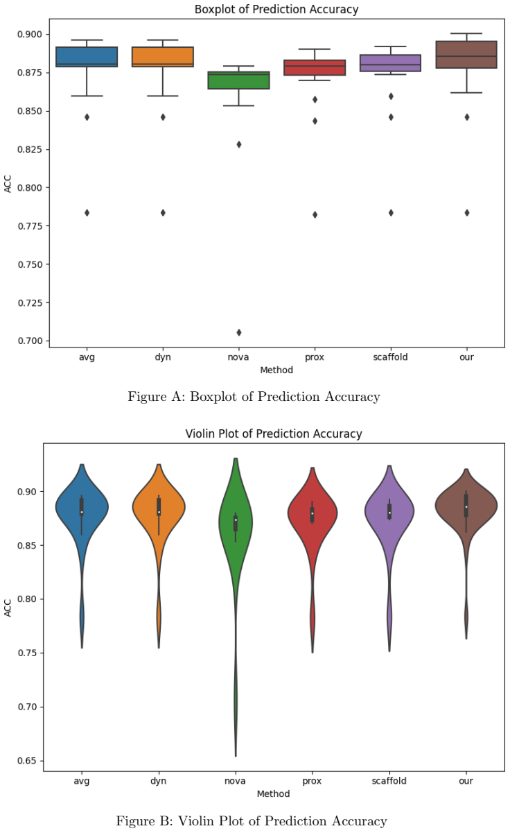
In the reported experiments, AMSFL reaches 89 percent accuracy in about 49 seconds, with a per-round time of 0.58 seconds, compared with slower per-round times for several baselines.

Reading between the lines

Editorial extensions of the paper, not claims the author makes directly.

A natural extension is to treat GDA as a generic drift estimator that could also be used to re-weight aggregation or to design proximal penalties, not just to set local step counts.
The same per-client step-allocation rule could be applied when the budget is energy or bandwidth rather than wall-clock time, since the cost parameter can be interpreted broadly.
If the strong-convexity assumption used in the proof is dropped, the residual bound may fail to hold on typical deep-network objectives, so the experimental validation would need to be repeated outside the convex regime.

Share X Bluesky LinkedIn Reddit HN

Editorial analysis

A structured set of objections, weighed in public.

Desk editor's note, referee report, and a circularity audit.

Desk Editor's Note

read the letter

Colleague,

You'll want to know before reading further: the GDA trick is a standard finite-difference Hessian-vector product approximation, and the idea of adapting local steps is not new; the only genuinely new piece is the greedy scheduler, which is a plausible heuristic. But the paper's advertised theory doesn't survive contact with its own equations. Theorem 3.4 is simply wrong — the KKT conditions give t_i = O(c_i/ω_i), not O((1/c_i)^{1/2}), and the objective is increasing in every t_i, so the greedy algorithm that saturates the budget is maximizing the error cost, not minimizing it. That's an internal contradiction, not a matter of taste.

To give credit where it's due: the paper is clearly written, the error recursion in Eq. (8) is a reasonable way to describe the drift, and the experimental comparison on NSL-KDD (though single-dataset) shows the heuristic does something sensible, beating fixed-step baselines in wall-clock time. The author also pays attention to related work and doesn't overstate the significance. So the empirical part might have some use.

But the soft spots are load-bearing, not cosmetic. Theorem 3.1 is more of a restatement than a proof — the cross terms are never bounded. Theorem 3.2's proof invokes strong convexity without listing it in A1–A4; typical deep networks aren't strongly convex. Proposition 3.3's proof needs Hessian Lipschitz continuity, which L-smoothness of the gradient does not imply. And Theorem 3.4's derivation of t* ∝ 1/sqrt(c_i) is the solution to minimizing Σ a_i/t_i, not the quadratic objective in Eq. (10). So the theoretical foundation of the step-allocation mechanism is unsupported.

The bottom line: as a heuristic paper with a corrected — or removed — theory section, there might be something here for practitioners working on resource-constrained federated learning. As written, the central claims don't hold. I wouldn't cite it, and I wouldn't send grad students to it for a template. It's borderline for a serious referee; the errors are specific enough that a careful referee could quickly flag them, so I'd lean yes to sending it out, but the expected outcome is major revision or rejection. If the author removes the false optimality claim and repositions the scheduler as a heuristic with empirical backing, it could be a minor workshop paper.

Recommendation: engage with it if you want a clear example of a KKT derivation gone wrong, but don't build on it.

Referee Report

5 major / 5 minor

Summary. The paper proposes GDA, a first-order approximation of local update drift, and AMSFL, a federated learning algorithm that uses the resulting error model to allocate local steps under a time budget. The authors derive an error recursion, a convergence bound, an approximation-error bound, and an optimal step-allocation formula, and report experiments on NSL-KDD showing improved accuracy and runtime over six baselines.

Significance. The problem of modeling local drift without second-order information and of adapting local steps under resource constraints is well motivated. If the theoretical claims were correct, the paper would make a useful contribution: the GDA error model is computationally cheap, and the allocation problem is practically relevant. However, the paper's central theoretical results are not established: the convergence proof relies on an unstated strong-convexity assumption, the GDA approximation proof assumes Hessian Lipschitz continuity and is circular with assumption A3, and the optimal-allocation theorem is algebraically incorrect. Since the adaptive mechanism in the experiments is based on this theorem, the empirical results do not validate the proposed framework as presented.

major comments (5)

[Section 3.3, Eq. (9), proof A.1] The proof of Theorem 3.1 expands ||e(k+1)||^2 but never bounds the drift cross term -2η⟨e(k), Σ_i ω_i Δ_i^{(t_i)}⟩ or the norm of the drift sum; the stated inequality with Δ_k therefore does not follow from the derivation. The later attempt in A.2 to control these terms introduces coefficients that do not match the Δ_k defined in the main text.
[Section 3.3, Theorem 3.2, proof A.2] The proof requires the global objective to be μ-strongly convex in order to assert ⟨e(k), Σ_i ω_i t_i ∇F_i(w(k))⟩ ≥ μE||e(k)||^2. Strong convexity is not among assumptions A1–A4 and is not satisfied by typical deep-network losses used in the experiments. Without this assumption the coefficient (1-θ) in the linearized recursion cannot be obtained, and the limsup bound is unsupported.
[Section 3.3, Proposition 3.3, proof A.3] The proof uses the Lipschitz continuity of ∇^2F, i.e., ||∇^2F(w+tδ)-∇^2F(w)|| ≤ Lt||δ||, which is not a consequence of L-smoothness of ∇F and is not stated among A1–A4. Moreover, assumption A3 is exactly the statement of Proposition 3.3, so the proposition cannot serve as an independent justification of A3; the argument is circular.
[Section 3.3, Theorem 3.4, Eq. (22)–(23)] The KKT stationarity condition gives t_i = 1/2 − α/β − λc_i/(βω_i), which is affine in c_i/ω_i and does not have the form (1/c_i)^{1/2}. In the large-t_i quadratic case min Σ(βω_i/2)t_i^2 subject to Σ c_i t_i ≤ S, stationarity yields t_i ∝ c_i/ω_i, not t_i ∝ (1/(c_iω_i))^{1/2}. The inverse-square-root allocation is the solution of a different objective of the form Σ a_i/t_i. The theorem as stated is therefore false.
[Section 3.4, Algorithm 1 and Eq. (10)] Because α,β>0 and t_i≥1, the objective in Eq. (10) is increasing in every t_i; under the inequality constraint Σ(c_i t_i + b_i) ≤ S the unconstrained minimum is t_i=1 for all i. Algorithm 1, which greedily adds steps until the budget is saturated, is maximizing rather than minimizing this objective. Thus the step-allocation mechanism used in the experiments is not grounded in the paper's error model.

minor comments (5)

[Section 3.3] The symbol Δ_k is used both for the aggregate bound η^2G^2E^2 + η^2L^2G^2D^2_k and, in proof A.2, for constants involving G_k and D_k; please use distinct notation.
[Section 3.4] In Eq. (10), α = 2η√µGk refers to µ and Gk that are not defined in the assumptions; if µ is meant to be the strong-convexity constant, it should be introduced in Section 3.3.
[Section 4] The enumeration 'Theorem 3.2–3.3' and 'Proposition 3.3' is confusing because Proposition 3.3 was already stated in Section 3.3; consider renumbering.
[Section 5] Tables 1 and 2 report no standard deviations or confidence intervals, and the model architecture, optimizer hyperparameters, and client partitioning are not specified, which limits reproducibility.
[Throughout] There are several typographical issues, including the repeated word 'a novelerror' in the introduction and missing spaces in theorem statements; a careful proofreading is needed.

Circularity Check

2 steps flagged · score 4.0 of 10

Mild circularity: GDA's approximation result restates its own assumption, and Theorem 3.4's advertised adaptive allocation is an imported inverse-square-root formula rather than a consequence of the paper's KKT equations.

self definitional [Section 3.3, Assumption A3; Proposition 3.3; Appendix A.3]
"(A3) Gradient difference approximation (GDA): ||∇2Fi(w) · δ − (∇Fi(w + δ) − ∇Fi(w))|| ≤ L/2 ||δ||2. ... Proposition 3.3 (Approximation Error of GDA). Let Fi be twice differentiable and L-smooth. Then for any update δ: ||∇2Fi(w) · δ − (∇Fi(w + δ) − ∇Fi(w))|| ≤ L/2 ||δ||2. ... Since ∇F is L-Lipschitz, it follows that ∇2F is also bounded in operator norm: ||∇2F(w + tδ) − ∇2F(w)|| ≤ Lt||δ||."

Proposition 3.3 is the same inequality as assumption A3, restated verbatim as a proved result. The proof in Appendix A.3 needs a Hessian-Lipschitz bound of the form ||∇2F(w+tδ)-∇2F(w)|| ≤ Lt||δ||, which is not a consequence of the stated L-smoothness assumption A1 and is not listed among A1-A4. Thus the GDA approximation error that Theorems 3.1-3.2 rely on is not independently established; the paper assumes the bound and then presents the same bound as its own proposition.
renaming known result [Theorem 3.4; Appendix A.4, Steps 2-3]
"This leads to a standard quadratic resource allocation problem: min Σ_i a_i t_i^2, s.t. Σ_i c_i t_i ≤ S, where a_i = βω_i/2. The classical solution is: t∗_i ∝ (1/(c_i a_i))^{1/2} = (1/(c_iω_i))^{1/2}."

The KKT equation in the same proof, ∂L/∂t_i = αω_i + βω_i(2t_i−1)/2 + λc_i = 0, gives t_i = 1/2 + (−αω_i−λc_i)/(βω_i), an affine function of c_i/ω_i. Minimizing the displayed quadratic cost Σ a_i t_i^2 under Σ c_i t_i ≤ S gives t_i* ∝ c_i/a_i, not ∝ 1/√(a_i c_i). The inverse-square-root formula is the known solution to minimizing Σ a_i/t_i, a different objective. The paper therefore imports a known allocation formula and relabels it as the solution of its own quadratic error model, so the advertised client-specific adaptive step sizes are not derived from the stated optimization.

full rationale

The empirical section is self-contained: AMSFL is compared against FedAvg, FedProx, SCAFFOLD, and others on NSL-KDD, and no benchmark numbers are fitted into the theory. There is no self-citation chain or uniqueness theorem borrowed from the authors. The main convergence theorem is conditional on explicit assumptions A1-A4, and although the proof silently adds µ-strong convexity (not in A1-A4 and not satisfied by typical deep networks), that is an assumption gap rather than circularity. The clearest circular step is Proposition 3.3 duplicating assumption A3, including a proof that smuggles in Hessian-Lipschitz continuity, so the GDA approximation error is not independently justified. Additionally, Theorem 3.4's advertised allocation t*_i ∝ 1/√(c_i ω_i) is not a consequence of the KKT equations supplied in Appendix A.4; the equations yield an affine allocation, and the quadratic large-t_i problem yields t_i ∝ c_i/ω_i. The inverse-square-root formula is the optimum of a different reciprocal-cost problem and is imported as a 'classical solution.' This is a serious derivation defect, but it is more an internal inconsistency than a fit-renamed-as-prediction or a self-citation chain, so the circularity score is moderate rather than extreme.

Assumptions & free parameters 2 free parameters · 6 assumptions · 0 invented entities

The central convergence and allocation results rest on Assumptions A1-A4 plus two unstated conditions: strong convexity and Hessian Lipschitz continuity. The GDA bound (A3) and drift bound (A4) are essentially the conclusions the theorems repackage. No new physical entities are introduced; the only free constants are alpha and beta, whose values are not reported.

free parameters (2)

alpha (convergence-driven term) = not reported
Used in Eq. (10) and greedy Algorithm 1; depends on eta, mu, and G and is not specified, so the scheduler is not reproducible.
beta (curvature-drift penalty) = not reported
Defined as (1/2) eta^2 L^2 G^2 in Section 3.4; L, G, and eta are unknown in experiments, making the allocation sensitive to uncalibrated constants.

assumptions (6)

domain assumption A1: Each local loss F_i is L-smooth.
Standard smoothness assumed in Section 3.3; used throughout the error bounds.
domain assumption A2: Gradient norms are bounded: ||grad F_i(w)|| <= G.
Used to bound drift terms, e.g., Delta_k and D^2_k.
ad hoc to paper A3: GDA error bound ||grad^2 F_i(w) delta - (grad F_i(w+delta)-grad F_i(w))|| <= (L/2)||delta||^2 is assumed, then independently 'proved' in Prop 3.3.
The bound is needed for GDA's justification; the proof uses an unstated Hessian Lipschitz assumption.
ad hoc to paper A4: Local drift accumulation ||Delta_i^(t_i)|| <= (LG/2) t_i(t_i-1).
This is exactly the O(t^2) drift that produces the D^2_k term in the global error bound; it is assumed, not derived.
ad hoc to paper Unstated strong convexity of global objective F (mu > 0).
Needed in Appendix A.2 to get the descent coefficient 2 eta mu E; not listed in Assumptions A1-A4.
ad hoc to paper Hessian Lipschitz continuity in Prop 3.3 proof.
The proof bounds ||grad^2 F(w+t delta)-grad^2 F(w)|| by L t ||delta||, which requires Lipschitz Hessian, not merely L-smooth gradients.

how reviews work

0 comments

Cite this review

Pith. "Pith review of AMSFL: Adaptive Multi-Step Federated Learning via Gradient Difference-Based Error Modeling." pith.science (2026). https://pith.science/paper/PLPDLBU2

@misc{pith2026250521695,
  author       = {Pith},
  title        = {Pith review of: AMSFL: Adaptive Multi-Step Federated Learning via Gradient Difference-Based Error Modeling},
  year         = {2026},
  howpublished = {\url{https://pith.science/paper/PLPDLBU2}},
  note         = {Machine review of arXiv:2505.21695}
}

read the original abstract

Federated learning faces critical challenges in balancing communication efficiency and model accuracy. One key issue lies in the approximation of update errors without incurring high computational costs. In this paper, we propose a lightweight yet effective method called Gradient Difference Approximation (GDA), which leverages first-order information to estimate local error trends without computing the full Hessian matrix. The proposed method forms a key component of the Adaptive Multi-Step Federated Learning (AMSFL) framework and provides a unified error modeling strategy for large-scale multi-step adaptive training environments.

Figures

Figures reproduced from arXiv: 2505.21695 by the authors.

Discussion (0). Sign in to comment.

Reference graph

Works this paper leans on

11 extracted references · 11 canonical work pages

[1]

Federated learning based on dynamic regularization

Durmus Alp Emre Acar, Yue Zhao, Rafael Navarro, Matthew Mattina, Paul Whatmough, and Venkatesh Saligrama. Federated learning based on dynamic regularization. In International Conference on Learning Representations (ICLR) , 2021

work page 2021
[2]

Altomare, D

V. Altomare, D. Thakur, A. Guzzo, et al. Client specific dynamic aggregation for non-iid federated learning. In Proceedings of the 2024 IEEE International Conference on Big Data (BigData), pages 7622–7631. IEEE, 2024

work page 2024
[3]

Scaffold: Stochastic controlled averaging for federated learning

Sai Praneeth Karimireddy, Satyen Kale, Mehryar Mohri, Sashank Reddi, Sebastian Stich, and Ananda Suresh. Scaffold: Stochastic controlled averaging for federated learning. In Proceedings of ICML , pages 5132–5143, 2020

work page 2020
[4]

Mime: Mimicking centralised stochastic algorithms in federated learning

Sai Praneeth Karimireddy, Sebastian U Stich, and Martin Jaggi. Mime: Mimicking centralised stochastic algorithms in federated learning. In International Conference on Machine Learning, pages 4653–4663, 2021

work page 2021
[5]

Federated optimization in heterogeneous networks

Tian Li, Anit Kumar Sahu, Ameet Talwalkar, and Virginia Smith. Federated optimization in heterogeneous networks. Proceedings of Machine Learning and Systems , 2:429–450, 2020

work page 2020
[6]

Communication- efficient learning of deep networks from decentralized data

Brendan McMahan, Eider Moore, Daniel Ramage, and Blaise Hampson. Communication- efficient learning of deep networks from decentralized data. In Proceedings of the 20th In- ternational Conference on Artificial Intelligence and Statistics (AISTATS) , pages 1273–1282. PMLR, 2017

work page 2017
[7]

Communication-efficient distributed optimization using an approximate newton-type method

Ohad Shamir and Nathan Srebro. Communication-efficient distributed optimization using an approximate newton-type method. In Proceedings of the 31st International Conference on Machine Learning, pages 1000–1008, 2014. 17

work page 2014
[8]

Local sgd converges fast and communicates little

Sebastian U Stich. Local sgd converges fast and communicates little. In International Confer- ence on Learning Representations (ICLR) , 2019

work page 2019

Show all 11 references

[9]

Tackling the objective inconsistency problem in heterogeneous federated optimization

Jianyu Wang, Qiang Liu, Hongyi Liang, Gauri Joshi, H Vincent Poor, Anit Kumar Sahu, and Ameet Talwalkar. Tackling the objective inconsistency problem in heterogeneous federated optimization. In NeurIPS, pages 7611–7623, 2020

2020
[10]

Op- timizing federated learning on non-iid data with reinforcement learning

Jun Wang, Mikhail Yurochkin, Yuekai Sun, Dimitris Papailiopoulos, and Yasin Khazaeni. Op- timizing federated learning on non-iid data with reinforcement learning. In NeurIPS Workshop on Federated Learning, 2020

2020
[11]

Disco: Distributed optimization for self-concordant empirical loss

Yuchen Zhang and John Duchi. Disco: Distributed optimization for self-concordant empirical loss. In Proceedings of the 32nd International Conference on Machine Learning, pages 362–370, 2015. 18

2015

Pith tools

Reviewed August 7, 2026 · model on record in the stance chip above.

[1] [1]

Federated learning based on dynamic regularization

Durmus Alp Emre Acar, Yue Zhao, Rafael Navarro, Matthew Mattina, Paul Whatmough, and Venkatesh Saligrama. Federated learning based on dynamic regularization. In International Conference on Learning Representations (ICLR) , 2021

work page 2021

[2] [2]

Altomare, D

V. Altomare, D. Thakur, A. Guzzo, et al. Client specific dynamic aggregation for non-iid federated learning. In Proceedings of the 2024 IEEE International Conference on Big Data (BigData), pages 7622–7631. IEEE, 2024

work page 2024

[3] [3]

Scaffold: Stochastic controlled averaging for federated learning

Sai Praneeth Karimireddy, Satyen Kale, Mehryar Mohri, Sashank Reddi, Sebastian Stich, and Ananda Suresh. Scaffold: Stochastic controlled averaging for federated learning. In Proceedings of ICML , pages 5132–5143, 2020

work page 2020

[4] [4]

Mime: Mimicking centralised stochastic algorithms in federated learning

Sai Praneeth Karimireddy, Sebastian U Stich, and Martin Jaggi. Mime: Mimicking centralised stochastic algorithms in federated learning. In International Conference on Machine Learning, pages 4653–4663, 2021

work page 2021

[5] [5]

Federated optimization in heterogeneous networks

Tian Li, Anit Kumar Sahu, Ameet Talwalkar, and Virginia Smith. Federated optimization in heterogeneous networks. Proceedings of Machine Learning and Systems , 2:429–450, 2020

work page 2020

[6] [6]

Communication- efficient learning of deep networks from decentralized data

Brendan McMahan, Eider Moore, Daniel Ramage, and Blaise Hampson. Communication- efficient learning of deep networks from decentralized data. In Proceedings of the 20th In- ternational Conference on Artificial Intelligence and Statistics (AISTATS) , pages 1273–1282. PMLR, 2017

work page 2017

[7] [7]

Communication-efficient distributed optimization using an approximate newton-type method

Ohad Shamir and Nathan Srebro. Communication-efficient distributed optimization using an approximate newton-type method. In Proceedings of the 31st International Conference on Machine Learning, pages 1000–1008, 2014. 17

work page 2014

[8] [8]

Local sgd converges fast and communicates little

Sebastian U Stich. Local sgd converges fast and communicates little. In International Confer- ence on Learning Representations (ICLR) , 2019

work page 2019