REVIEW 3 major objections 4 minor 17 references
A new asymmetric $\epsilon$-insensitive pinball loss function based support vector quantile regression model
T0 review · 3 major / 4 minor · reviewed 2026-08-14 · deepseek-v4-flash
Pith's one-line read This paper proposes an asymmetric epsilon-insensitive pinball loss that keeps a fixed-width quantile tube and restores sparsity in support vector quantile regression.
desk verdict The proposed loss is exactly Park and Kim's loss under a tau-dependent rescaling of epsilon, so the novelty claim and the reported improvements are artifacts of the parameterization and the epsilon grid. read the letter →
The pith
A machine-rendered reading of the paper's core claim, the machinery that carries it, and where it could break.
The reading
What carries the argument
The central object is the proposed asymmetric epsilon-insensitive pinball loss in Eq. (5): $L^\epsilon_\tau(u)=\max(-(1-\tau)(u+\tau\epsilon),0,\tau(u-(1-\tau)\epsilon))$, where $u$ is the signed residual $y-(w^\top\varphi(x)+b)$ and $\tau\in(0,1)$ is the target quantile. It combines a one-sided upper arm with slope $\tau$ that activates above $(1-\tau)\epsilon$ and a one-sided lower arm with slope $-(1-\tau)$ that activates below $-\tau\epsilon$, joined by a flat zero-cost tube of total width $\epsilon$. This machinery produces sparsity: inside the tube the dual variables $\alpha_i,\beta_i$ vanish, boundary points determine the bias, and the final quantile regressor is built only from boundary and outside points, with contributions weighted in the ratio $(1-\tau)$ to $\tau$.
What would settle it
For one of the paper's datasets, solve the earlier epsilon-insensitive SVQR with its epsilon parameter multiplied by $\tau(1-\tau)$ and compare the resulting regression functions and error tables with the proposed model across the same epsilon grid; identical outputs would show the two formulations coincide.
Extended reading notes
Core claim
The central claim is that the loss $L^\epsilon_\tau(u)=\max(-(1-\tau)(u+\tau\epsilon),0,\tau(u-(1-\tau)\epsilon))$ is the first asymmetric epsilon-insensitive pinball loss that extends the epsilon-insensitive idea faithfully: the insensitive zone has total width $\epsilon$ regardless of $\tau$, and the $\tau$ value only decides how that width is divided between the region above and below the regressor. Training points whose residuals fall inside this asymmetric tube contribute zero loss and drop out of the dual solution, restoring sparsity to support vector quantile regression, which the standard pinball loss lacks. With $\epsilon=0$ the model reduces to the standard support vector quantile regression model; with nonzero $\epsilon$ the paper reports lower root-mean-square error and coverage error than the standard, sparse, and earlier epsilon-insensitive models on the datasets tested.
Load-bearing premise
The comparison assumes the proposed loss is genuinely different from a previously proposed epsilon-insensitive quantile regression loss, so that using the same numeric epsilon for both is a fair test; if the two losses are the same family after rescaling epsilon, the reported advantage is an artifact of the parameter grid.
Editorial extensions
If this is right
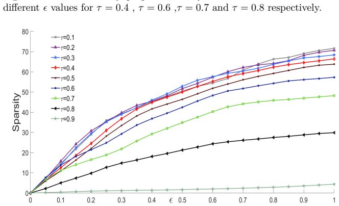
- The epsilon-SVQR dual solution has many zero coefficients, so predictions use only boundary and outside points rather than the entire training set.
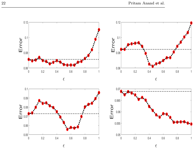
- For a given quantile, the epsilon tube can be widened or narrowed without changing the quantile's asymmetry, and the paper's experiments tie the best epsilon value to the noise variance in the response.
- With epsilon set to zero, the model coincides with the standard SVQR, so the new model generalizes rather than replaces the existing formulation.
- Coverage error and sparsity both improve as epsilon grows in most of the paper's benchmark experiments, suggesting a practical trade-off between ignoring more points and maintaining quantile accuracy.
Reading between the lines
- Algebraically, the proposed loss is $\max(0, P_\tau(u)-\tau(1-\tau)\epsilon)$, which is exactly the loss of the earlier epsilon-insensitive quantile regression model with its own parameter set to $\tau(1-\tau)\epsilon$; the two models therefore form the same one-parameter family, so the claimed new family is a reparameterization.
- If that equivalence holds, the reported improvement over the earlier model likely reflects the effective tube widths the search grid happened to select rather than an intrinsic property; a matched-scale comparison would test this directly.
- A practical extension the paper leaves open is a data-driven rule for setting $\epsilon$, since the optimal value in the experiments grows with the noise variance in the response.
- The fixed-width property suggests interpreting $\epsilon$ as a noise-scale parameter shared across quantiles, which could simplify tuning when several quantile curves are estimated jointly.
Signed reviews
Editorial analysis
A structured set of objections, weighed in public.
Referee Report
Summary. The paper proposes an asymmetric ε-insensitive pinball loss function, L^ε_τ(u) = max(−(1−τ)(u+τε), 0, τ(u−(1−τ)ε)), for support vector quantile regression, and names the resulting model ε-SVQR. It derives the primal and dual quadratic programs, states a sparsity property via Proposition 1, and reports experiments on artificial and UCI datasets comparing ε-SVQR with standard SVQR, Sparse SVQR (Seok et al.), and Park-Kim SVQR. The abstract claims that the proposed loss is the first to extend the ε-insensitive approach to quantile regression 'in true sense', that it improves prediction significantly, and that it restores sparsity.
Significance. If the proposed loss were genuinely new, it would provide a convenient fixed-width asymmetric tube for quantile regression with sparsity and would constitute a meaningful contribution to the SVQR literature. However, as shown in the major comments, the loss is algebraically identical to the Park-Kim loss under a simple rescaling of the tube-width parameter, so the central novelty claim is not correct. The paper does contain a complete QP derivation and a broad experimental study, but the numerical comparisons with Park-Kim are not comparisons of different model families. The practical value of the paper reduces to a reparameterization of an existing loss, which does not support the claimed significance.
major comments (3)
- [Eq. (5) vs. Eq. (4)] The proposed loss in Eq. (5) is algebraically identical to the Park-Kim loss in Eq. (4) under the substitution ε_PK = τ(1−τ)ε. For u > (1−τ)ε, L^ε_τ(u) = τu − τ(1−τ)ε = P_τ(u) − ε_PK; for u < −τε, L^ε_τ(u) = −(1−τ)u − τ(1−τ)ε = P_τ(u) − ε_PK; and the flat interval [−τε, (1−τ)ε] equals the Park-Kim flat interval [−ε_PK/(1−τ), ε_PK/τ]. Since ε_PK is a free user parameter, the two loss families coincide exactly. This contradicts the paper's central claim (Abstract and Section 1) that the proposed loss extends the ε-insensitive idea to quantile regression 'in true sense' and that Park-Kim's loss has a different, τ-dependent width. The difference between the two formulations is purely a reparameterization of the tube width.
- [Proposition 1 (Section 3)] Proposition 1 states that α_i β_i = 0 for all i for ε ≥ 0, but it is false when ε = 0. At ε = 0, a training point whose residual is exactly zero satisfies both KKT conditions (23) and (24) with ξ_i = ξ*_i = 0, so both α_i and β_i can be positive. The proof adds (30) and (31) to obtain ξ*_i + ξ_i = −ε; at ε = 0 this equation is consistent with ξ_i = ξ*_i = 0, so the alleged contradiction disappears. Since the paper explicitly notes that the model reduces to standard SVQR at ε = 0, the sparsity classification into S1, S2, and S3 does not hold in that case, and the proposition's statement for all ε ≥ 0 is incorrect.
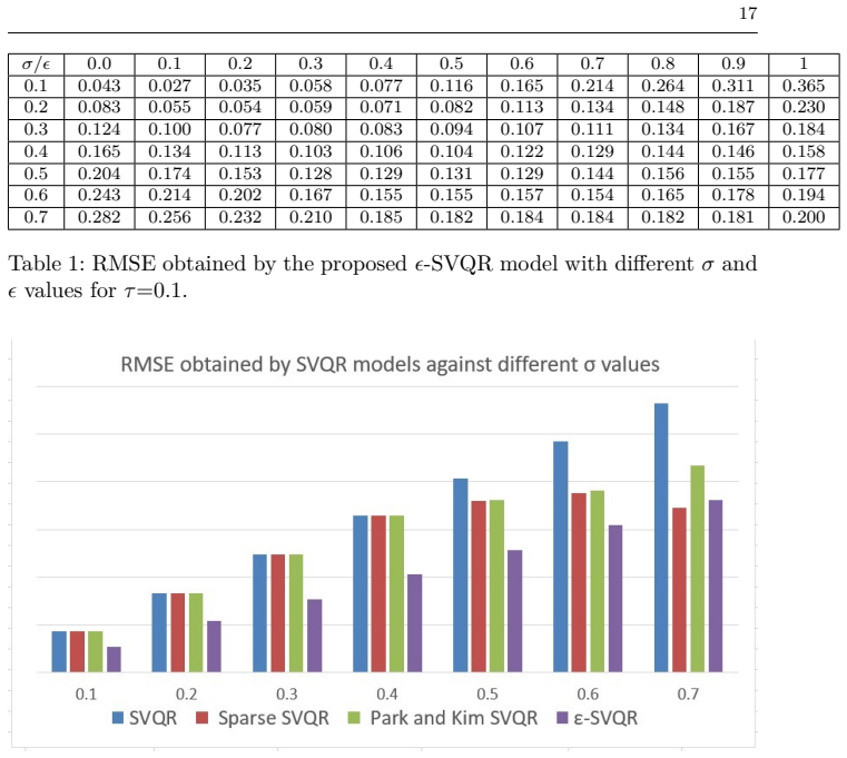
- [Tables 3, 6, 11, 12 and Section 4.2] The numerical comparisons with Park-Kim SVQR use the same numerical ε grid for both methods but do not account for the reparameterization ε_PK = τ(1−τ)ε. For example, at τ = 0.1 the proposed ε = 1 corresponds to Park-Kim ε_PK = 0.09, which is not in the stated search set {0, 0.1, 0.2, ...}. Thus the reported improvements of ε-SVQR over Park-Kim SVQR are at least partly artifacts of a mismatched ε grid, not evidence that the proposed model family is superior. The experiments in Section 4.2 and on the UCI datasets therefore do not support the abstract's claim of significant improvement over existing SVQR models.
minor comments (4)
- [Section numbering] The Introduction states that Section 5 contains numerical results and Section 6 concludes, but the actual sections are numbered 4 (Experimental Results) and 5 (Conclusion).
- [Eq. (16)] The notation in Eq. (16) is confusing because ξ_i and ξ*_i are reused before and after the rescaling ξ_i := ξ_i/τ and ξ*_i := ξ*_i/(1−τ); the derivation would be clearer with different symbols for the intermediate variables.
- [Throughout] There are many typographical errors, including 'Preposition' instead of 'Proposition', 'e-insensitive' instead of 'ε-insensitive', 'artifical' instead of 'artificial', and 'Traizines' instead of 'Triazines' in the UCI dataset name.
- [Section 4.2, discussion of Sparse SVQR] The statement that Sparse SVQR 'fails to control the effective width' of the ε-insensitive zone for low τ is a consequence of fixing ε numerically rather than a property of the model family; Seok et al.'s loss also has ε as a free tunable parameter.
Circularity Check
The proposed loss (5) is algebraically identical to Park and Kim's Eq (4) under ε_PK = τ(1−τ)ε; the claimed novelty and reported improvements rest on a reparameterization, not a new model.
-
renaming known result
[Section 1, Eq. (4) and Eq. (5); Section 3, primal and dual formulations (13)-(29)]
"ρϵ τ(u) =max(0,Pτ(u)) = { Pτ(u)−ϵ, if Pτ(u)>ϵ. 0, otherwise. (4) ... Lϵ τ(u) =max( −(1−τ)(u +τϵ), 0 , τ(u−(1−τ)ϵ) ) (5)"
For u > (1−τ)ε, L = τ(u − (1−τ)ε) = τu − τ(1−τ)ε; for u < −τε, L = −(1−τ)(u + τε) = Pτ(u) − τ(1−τ)ε; the flat interval is [−τε, (1−τ)ε]. This is exactly Park and Kim's max(0, Pτ(u) − ε_PK) with ε_PK = τ(1−τ)ε. Since ε_PK is a free user parameter, the two loss families coincide; the proposed loss is a reparameterization of Eq. (4), not a new asymmetric ε-insensitive extension. The dual problem (29) is the same dual under that substitution.
-
renaming known result
[Section 1, discussion of Park and Kim [14]; Section 4.2-4.3, Tables 3, 6, 7, 11]
"Similar to the e-insensitive pinball loss function of Seok et al.[13], the width of the ϵ-insensitive zone in the loss function of Park and Kim [14] also varies with the τvalues. ... Unlike other ϵ-insensitive loss functions, the overall width of the ϵ-zone in the proposed asymmetric ϵ-insensitive pinball loss function does not vary for different values of τ"
This contrast is an artifact of fixing a numeric ε across τ. Because ε_PK = τ(1−τ)ε is free, Park and Kim's tube can also have any fixed width; only the parameterization differs. The experiments give both methods the same ε grid, so for τ = 0.1 the proposed ε = 1 corresponds to ε_PK = 0.09, a value the Park-Kim grid was not allowed to use. The claimed 'significant improvement' is therefore forced by the choice of ε grid, not by a different model family.
full rationale
The paper's QPP derivation is internally self-contained, but its central novelty is not independent of prior work. Equation (5) is literally Park and Kim's Eq. (4) under the substitution ε_PK = τ(1−τ)ε; because ε is a user-tuned parameter, every proposed loss is already a Park-Kim loss. Consequently, the abstract's claim that earlier losses 'fail to extend the ε-insensitive approach for quantile estimation in true sense' and that the proposed loss creates a fixed-width asymmetric ε-zone is a reparameterization presented as a new model. The numerical comparisons in Tables 3, 6, 7, and 11 compare the same family using the same numeric ε grid, which for τ ≠ 0.5 gives the proposed method access to effective Park-Kim widths such as ε_PK = 0.09 that the Park-Kim grid excludes; the reported gains are a grid artifact. This is a renaming/known-result circularity rather than a self-citation chain, so the score is 8 rather than 10. Separately, Proposition 1's proof is invalid at ε = 0 because both multipliers can be positive when a residual lies exactly on a boundary, but that is a correctness issue, not a circularity one.
Assumptions & free parameters
free parameters (3)
- epsilon =
grid {0,0.1,0.2,...,2,2.5,3,...,5}; optimal values per dataset in Tables 1-14
- C (regularization) =
grid {2^i: i=-15,-9,...,9,15}; optimal values reported in Table 8 for AD2
- kernel width q =
same grid as C; optimal values in Table 8
assumptions (4)
- standard math The representer theorem: the optimal w lies in the span of kernel functions at training points and the bias term can be handled by the equality constraint.
- standard math Strong duality holds for the convex QP so the Wolfe dual is exact.
- domain assumption Minimizing the pinball loss estimates the true conditional quantile.
- domain assumption The RBF kernel with a single width q is suitable for all datasets.
Cite this review
Pith. "Pith review of A new asymmetric $\epsilon$-insensitive pinball loss function based support vector quantile regression model." pith.science (2026). https://pith.science/paper/PQQMAU33
@misc{pith2026190806923,
  author       = {Pith},
  title        = {Pith review of: A new asymmetric $\epsilon$-insensitive pinball loss function based support vector quantile regression model},
  year         = {2026},
  howpublished = {\url{https://pith.science/paper/PQQMAU33}},
  note         = {Machine review of arXiv:1908.06923}
}
abstract
In this paper, we propose a novel asymmetric $\epsilon$-insensitive pinball loss function for quantile estimation. There exists some pinball loss functions which attempt to incorporate the $\epsilon$-insensitive zone approach in it but, they fail to extend the $\epsilon$-insensitive approach for quantile estimation in true sense. The proposed asymmetric $\epsilon$-insensitive pinball loss function can make an asymmetric $\epsilon$- insensitive zone of fixed width around the data and divide it using $\tau$ value for the estimation of the $\tau$th quantile. The use of the proposed asymmetric $\epsilon$-insensitive pinball loss function in Support Vector Quantile Regression (SVQR) model improves its prediction ability significantly. It also brings the sparsity back in SVQR model. Further, the numerical results obtained by several experiments carried on artificial and real world datasets empirically show the efficacy of the proposed `$\epsilon$-Support Vector Quantile Regression' ($\epsilon$-SVQR) model over other existing SVQR models.
Figures


Figures from the paper (8 more)





Reference graph
Works this paper leans on
-
[1]
R Koenker , G Bassett , Regression quantiles, Econometrica Mathematical Reviews 46 pp 33-50 https://doi.org/10:1913643
-
[2]
R. Koenker. Quantile Regression, Cambridge University Press, 2005
work page 2005
-
[3]
Y Keming, RA Moyeed, Bayesian quantile regression, Statistics and Probability Letters 54.4(2001) pp 437-447
work page 2001
-
[4]
RJ Bosch, Y Ye, GG Woodworth, A convergent algorithm for quantile regression with smoothing splines, Computational Statistics and Data Analysis,19(1995) pp 613-630
work page 1995
-
[5]
K Yu , MC Jones, Local linear quantile regression, Journal of the American statistical Association 93.441 (1998) pp 228-237
work page 1998
-
[6]
Takeuchi, QV Le, TD Sears, AJ Smola, Nonparametric quantile estimation, Journal of Machine Learning Research, 7 (2006), pp 1231-1264
work page 2006
-
[7]
V Vapnik, S Golowich, A Smola, Support vector method for function approximation, regression estimation and signal processing, Advances in neural information processing systems, (1997) 281-287
work page 1997
-
[8]
H Drucker, CJ Burges, L Kaufman, AJ Smola, V Vapnik, Support vector regression machines, Advances in neural information processing systems (1997), pp 155-161
work page 1997
Show all 17 references
-
[9]
S Gunn, Support vector machines for classification and regression, ISIS technical report 14.1 (1998), pp 5-16
1998
-
[10]
V Vapnik Statistical learning theory , Vol 1 New York Wiley 1998
1998
-
[11]
I Takeuchi and T Furuhashi, Non-crossing quantile regressions by SVM, IEEE Interna- tional Joint Conference on Neural Networks (2004) Vol. 1, pp. 401-406
2004
-
[12]
T Hu, DH Xiang and DX Zhou , Online learning for quantile regression and support vector regression, Journal of Statistical Planning and Inference (2012), 142.12,3107-3122
2012
-
[13]
1 (2010), pp V1-438
KH Seok, D Cho, C Hwang, J Shim, Support vector quantile regression using asym- metric e-insensitive loss function, In Education Technology and Computer (ICETC), 2nd International Conference on Vol. 1 (2010), pp V1-438
2010
-
[14]
P Jinho, J Kim ,Quantile regression with an epsilon-insensitive loss in a reproducing kernel Hilbert space, Statistics and probability letters 81.1 (2011): 62-70
2011
-
[15]
CW Hsu , CJ Lin, A comparison of methods for multi class support vector machines, IEEE Transaction on Neural Networks,13 (2002) 415-425
2002
-
[16]
Q Xu, J Zhang, C Jiang, X Huang, Y He, Weighted quantile regression via support vector machine, Expert Systems with Applications, 42(13),(2015) pp 5441-5451
2015
-
[17]
CL Blake, UCI repository of machine learning databases, irvine, university of california, (1998), http://www. ics. uci. edu/˜ mlearn/MLRepository. html
1998
Reviewed August 14, 2026 · model on record in the stance chip above.
Discussion (0). Continue with ORCID to comment.