REVIEW 3 major objections 4 minor 29 references
Compression Method for Deep Diagonal State Space Model Based on $H^2$ Optimal Reduction
T0 review · 3 major / 4 minor · reviewed 2026-08-06 · deepseek-v4-flash
Pith's one-line read Finite-time H2 reduction shrinks diagonal state-space models to 1/32 size without accuracy loss.
desk verdict A real method for structure-preserving finite-time H2 reduction of diagonal SSMs, with a sound core, but the abstract's 'without sacrificing performance' claim is not backed by the paper's own multi-seed numbers. read the letter →
The pith
A machine-rendered reading of the paper's core claim, the machinery that carries it, and where it could break.
The reading
What carries the argument
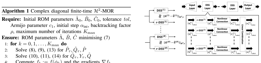
The central object is the finite-time H2 norm ∥G−Ĝ∥_{H2,τ}, defined via finite-time Gramians Pτ and Qτ (integrals of the matrix exponentials $e^{{At}}$BB*$e^{{A*t}}$ and $e^{{A*t}}$C*$Ce^{{At}}$ over [0,τ]), together with the inequality (5) that bounds the maximum output error over [0,τ] by this norm times the input energy. The paper reduces the model-order-reduction problem to minimizing the surrogate f(Λ̂,B̂,Ĉ) from Proposition 1, then derives gradients for the complex diagonal parameters (Theorem 1) and runs a backtracking descent (Algorithm 1) that enforces stability. The DSS-EXP parameterization (15) makes stability automatic and B constant, simplifying the gradient updates to the chain-rule forms in Proposition 2.
What would settle it
A concrete check would be to take a pre-trained DDSSM where the proposed fH2 ROM has lower finite-time H2 error than an iBT ROM, re-train both from those initializations, and observe that the fH2-initialized network ends up with equal or lower accuracy than the iBT-initialized one across many seeds, which would break the assumed link between the H2 surrogate and final performance. Alternatively, a controlled experiment varying the inference length Linf around the training horizon τ could test whether the method's advantage disappears when the actual inference horizon differs from the τ used in the reduction.
Extended reading notes
Core claim
On the paper's own terms, the central discovery is that finite-time H2-optimal model order reduction—not the infinite-time H∞-oriented balanced truncation used in earlier work—is the better reduction criterion for compressing the linear DSS blocks inside deep sequence models. Working over the actual input horizon τ = LΔ, the algorithm (gradient descent on a nonconvex objective with stability enforcement) produces reduced-order models with lower finite-time H2 error than balanced truncation, and these models, when used as initializations for re-training the deep model, yield better final accuracy. In the strongest reported configuration, a reduced DSS with r=2 (state-space parameters 1/32 of the original N=64) reaches 84.51% on IMDb, exceeding both the full model's 84.49% and all compared compression baselines; a paired t-test over 10 seeds gives t=3.30, p=0.0093 against infinite-time BT at r=2.
Load-bearing premise
The whole approach assumes that reducing the linear part's finite-time H2 error, as bounded by inequality (5), actually translates into a better final accuracy after the nonlinear deep model is re-trained; the paper does not model how gating, channel mixing, or re-training dynamics respond to the reduced initialization.
Editorial extensions
If this is right
- Compressing a diagonal SSM's state dimension from 64 to 2 (1/32 of the parameters) can match or exceed the full model's IMDb accuracy, with 84.51% versus 84.49%.
- Finite-time H2-optimal ROMs outperform infinite-time balanced truncation as initializations for re-training, and the r=2 gap is statistically significant (p=0.0093 over 10 seeds).
- The same pipeline generalizes to ListOps, where the r=4 fH2 configuration reaches 60.90% versus 59.75% for iBT, surpassing the pre-trained N=64 baseline of 60.50%.
- The algorithm preserves the DSS-EXP structure (complex diagonal, stable), so the compressed model retains the fast FFT-based training and inference of the original architecture.
- Since the gradient algorithm is parameterized by reduced dimension r and horizon τ, a user can trade accuracy against size by choosing r and can match the inference horizon τ to the actual input length.
Reading between the lines
- If the link between finite-time H2 error and re-trained accuracy holds generally, the same reduction could be applied to other structured state-space architectures, such as selective or input-dependent SSMs, provided the optimization is adapted to non-diagonal dynamics.
- The method suggests that pruning for sequence models should measure a component's contribution over the actual truncated input window rather than over infinite time, since real inputs are finite in practice.
- A testable extension is to freeze the reduced ROM entirely and re-train only the nonlinear mixing parts, which would cut training cost further; the paper's before/after columns suggest performance depends strongly on re-training, so freezing might degrade accuracy.
Signed reviews
Editorial analysis
A structured set of objections, weighed in public.
Referee Report
Summary. The paper proposes a finite-time H2 model order reduction (MOR) method for the diagonal state space models used inside deep diagonal state space models (DDSSMs). The proposed optimization problem preserves the complex diagonal structure and stability of the original DSS models, and the authors derive gradients for the complex-valued parameters and give a gradient-based algorithm with a stability-preserving line search. The method is embedded in the compression pipeline of [14]: pre-train an N=64 DSSEXP model, reduce it to r dimensions with the proposed H2 MOR, and re-train the compressed deep model. Experiments on the IMDb and ListOps LRA tasks compare the proposed fH2 method with balanced truncation variants, random initialization, and the original model, and report that fH2 attains 84.51% at r=2 versus a 84.49% baseline while reducing SSM parameters to 1/32. The paper claims that this compression outperforms BT-based compression and does not sacrifice the performance of the original model.
Significance. If the headline claims are supported, the paper is a useful systems-theoretic contribution: it extends time-limited H2-optimal MOR to complex diagonal state space layers, provides explicit gradients, and demonstrates an application to deep SSM compression. The formulation of the objective as the true finite-time H2 error of the transfer function is not circular, and the reported convergence plots show that the algorithm reduces the objective relative to BT and random initializations. The paired t-test against BT at r=2 is a good practice. However, the central parity claim ('without sacrificing performance') is not supported by the statistics reported in the paper: the multi-seed means in the appendices are below the original-model baseline, and no significance test against the original model is given. The significance of the contribution is therefore conditional on a revised statistical analysis or a more modest claim.
major comments (3)
- [Abstract; Section IV-D; Appendix G] The abstract and conclusion claim that compression to r=2 ('1/32 of the original') can be done 'without sacrificing the performance of the original models.' The evidence for this parity claim is not reported. Table I gives a single accuracy of 0.8451 for fH2(LDelta) at r=2 against a pretrained N=64 baseline of 0.8449, with no error bars or seed count. The multi-seed results in the same paper contradict that point estimate: Appendix G reports a 10-seed mean of 0.84184 for fH2-fBT at r=2, which is 0.00306 below the baseline, and Table III reports a five-seed mean of 0.8422. No paired significance test against the original N=64 model is provided; the t-tests in Table IV only compare fH2-fBT with iBT and with random initialization. Please add a paired test of fH2 versus the original model, or revise the claim to one that does not assert parity.
- [Table I; Appendix F] The discrepancy between the Table I result and the multi-seed means must be reconciled. Table I appears to be based on a single seed, while Table III and Appendix G average over five and ten seeds. If the Table I entry is one favorable seed, the 0.02 percentage point advantage over the baseline is within seed noise and should not be presented as 'outperforming' or 'without sacrificing performance.' The paper should report means and standard deviations for Table I, or clearly state that Table I is a representative run and base claims on the multi-seed results.
- [Section II-C and Section IV-D] Inequality (5) bounds the difference between the linear outputs y and y-hat before any re-training. The final accuracies in Table I and Table III are obtained after re-training the full nonlinear deep model with gating and channel mixing. The link between lower finite-time H2 error of the linear ROM and higher re-trained accuracy is therefore empirical, not derived. The paper should state this limitation explicitly and, if possible, provide evidence across seeds that lower linear H2 error is predictive of re-trained accuracy; currently the argument is stronger than the theory supports.
minor comments (4)
- [Algorithm 1] In line 3 of Algorithm 1, the text says 'Solve (10), (11), (14) for Q_hat_tau, Y_tau, Q_hat,' but equations (10), (11), and (14) define X_tau, Y_tau, and X, respectively. Please correct the variable names in the algorithm.
- [Abstract; Section IV] The abstract says 'the LRA benchmark results,' but the paper evaluates only two LRA tasks (IMDb and ListOps). Please say 'on two LRA tasks' or report all five LRA datasets to match the wording.
- [Table II] The dash entries for fH2(LDelta) at r=32 and r=16 in the ListOps table are not explained in the ListOps subsection. Please add a note that the ROMs are omitted because finite-time BT produced unstable initial models or the method was not run for that configuration.
- [Appendix G] The power analysis in Appendix G is reasonable, but the paper should state the exact 10-seed means and standard deviations for each method in the same table as the t-test results, so that the reader can see the difference from the original-model baseline without cross-referencing Table III and the text.
Circularity Check
No exhibit-able circular reduction: the H2-MOR objective is a genuine transfer-function error norm; [14] (co-author) supplies the pipeline and baseline but is non-load-bearing. The statistical parity claim is fragile, but that is a correctness risk, not a circularity.
full rationale
The derivation chain is self-contained and I find no circular step to exhibit. The core optimization (problems (6)/(12)) directly minimizes ||G - Ĝ||²_{H2,τ}, a mathematically defined finite-time H2 error between the original and reduced transfer functions; no downstream accuracy enters the objective, and the horizon τ is reported for all three choices (L∆, L, 10L) rather than fitted to the benchmark. The gradients (Theorem 1) and the DSS EXP chain rule (Proposition 2) are proved in the appendix starting from external, non-overlapping results [19]-[21], [27], so the derivation does not reduce to its own inputs. The benchmark claim (fH2 vs iBT at r=2) is a genuine paired re-training comparison on the external IMDb task with 10 shared seeds (t=3.30, p=0.0093), and Appendix F shows fH2 also outperforms random-stable initialization, so the advantage is measured rather than constructed. The paper does borrow the three-stage pipeline, the BT baseline, and the BT initializer from [14] (co-author K. Sato), but this self-citation is not load-bearing: it supplies the experimental setup, while the new MOR algorithm and its optimality properties are developed independently and robustness to initialization is tested in-paper. The weakest premise, that the linear finite-time H2 error bound (5) governs the accuracy of the re-trained nonlinear model (Sections II-C and IV-D), is an empirical assumption that the paper itself evaluates; even if it is imperfect, it is not a definitional loop. The abstract's 'without sacrificing the performance of the original models' is statistically under-supported: the 10-seed mean for fH2-fBT-ROM at r=2 is 0.84184, below the N=64 baseline of 0.8449, and no significance test against the original model is reported (Table I versus Appendix G). That is a correctness or over-claiming concern, explicitly not a circularity one. Score 2 reflects the single minor, non-load-bearing self-citation.
Assumptions & free parameters
free parameters (4)
- Reduced order r =
2, 4, 8, 16, 32 in experiments; headline result at r=2
- MOR time horizon tau =
L*Delta, L, 10L; L*Delta emphasized in the headline
- MOR optimization hyperparameters =
tol=1e-3, c1=1e-4, rho=0.5, Kmax=100, alpha_ini=1
- Random seeds for re-training =
10 seeds for the main t-test; 5 seeds in Appendix F
assumptions (4)
- standard math The finite-time Gramians P_tau and Q_tau are unique solutions of equations (2) and (3), requiring lambda_i + conjugate(lambda_j) != 0 for all eigenvalue pairs.
- standard math Time-limited H2 optimality conditions from [19]-[21] extend to complex diagonal state matrices.
- domain assumption The finite-time H2 output error of the linear SSM is a valid proxy for the final task accuracy of the full nonlinear deep model after re-training.
- domain assumption The DSSEXP parameterization Lambda = -exp(Lambda_re) + i*Lambda_im is used for both the original and reduced models, guaranteeing stability and simplifying the optimization.
Cite this review
Pith. "Pith review of Compression Method for Deep Diagonal State Space Model Based on $H^2$ Optimal Reduction." pith.science (2026). https://pith.science/paper/PRZZTKSL
@misc{pith2026250710078,
  author       = {Pith},
  title        = {Pith review of: Compression Method for Deep Diagonal State Space Model Based on $H^2$ Optimal Reduction},
  year         = {2026},
  howpublished = {\url{https://pith.science/paper/PRZZTKSL}},
  note         = {Machine review of arXiv:2507.10078}
}
abstract
Deep learning models incorporating linear SSMs have gained attention for capturing long-range dependencies in sequential data. However, their large parameter sizes pose challenges for deployment on resource-constrained devices. In this study, we propose an efficient parameter reduction method for these models by applying $H^{2}$ model order reduction techniques from control theory to their linear SSM components. In experiments, the LRA benchmark results show that the model compression based on our proposed method outperforms an existing method using the Balanced Truncation, while successfully reducing the number of parameters in the SSMs to $1/32$ without sacrificing the performance of the original models.
Figures


Reference graph
Works this paper leans on
-
[19]
Time-limited H2-optimal model order reduction,
P. Goyal and M. Redmann, “Time-limited H2-optimal model order reduction,” Applied Mathematics and Computation , vol. 355, pp. 184– 197, 2019
work page 2019
-
[21]
H2 Optimal Model Order Reduction Over a Finite Time Interval,
K. Das, S. Krishnaswamy, and S. Majhi, “ H2 Optimal Model Order Reduction Over a Finite Time Interval,” IEEE Control Systems Letters , vol. 6, pp. 2467–2472, 2022
work page 2022
-
[14]
Model Compression Method for S4 with Diagonal State Space Layers using Balanced Truncation,
H. Ezoe and K. Sato, “Model Compression Method for S4 with Diagonal State Space Layers using Balanced Truncation,” IEEE Access, 2024
work page 2024
-
[1]
A new approach to linear filtering and prediction problems,
R. E. Kalman, “A new approach to linear filtering and prediction problems,” 1960
1960
-
[2]
Long Range Lan- guage Modeling via Gated State Spaces,
H. Mehta, A. Gupta, A. Cutkosky, and B. Neyshabur, “Long Range Lan- guage Modeling via Gated State Spaces,” in International Conference on Learning Representations , 2023
work page 2023
-
[3]
X. Jiang, C. Han, and N. Mesgarani, “Dual-path Mamba: Short and Long-Term Bidirectional Selective Structured State Space Models for Speech Separation,” in ICASSP 2025 – IEEE International Conference on Acoustics, Speech and Signal Processing . IEEE, 2025, pp. 1–5
work page 2025
-
[4]
U-mamba: Enhancing long-range dependency for biomedical image segmentation,
J. Ma, F. Li, and B. Wang, “U-mamba: Enhancing long-range dependency for biomedical image segmentation,” arXiv preprint arXiv:2401.04722, 2024
arXiv 2024
-
[5]
Videomamba: State space model for efficient video understanding,
K. Li, X. Li, Y . Wang, Y . He, Y . Wang, L. Wang, and Y . Qiao, “Videomamba: State space model for efficient video understanding,” in European Conference on Computer Vision . Springer, 2024, pp. 237– 255
work page 2024
Show all 29 references
-
[6]
Hippo: Recurrent memory with optimal polynomial projections,
A. Gu, T. Dao, S. Ermon, A. Rudra, and C. R ´e, “Hippo: Recurrent memory with optimal polynomial projections,” in Advances in Neural Information Processing Systems , 2020, pp. 1474–1487
2020
-
[7]
Combining Recurrent, Convolutional, and Continuous-time Models with Linear State-Space Layers,
A. Gu, I. Johnson, K. Goel, K. Saab, T. Dao, A. Rudra, and C. R ´e, “Combining Recurrent, Convolutional, and Continuous-time Models with Linear State-Space Layers,” Advances in Neural Information Pro- cessing Systems, vol. 34, 2021
2021
-
[8]
Efficiently modeling long sequences with structured state spaces,
A. Gu, K. Goel, and C. R ´e, “Efficiently modeling long sequences with structured state spaces,” in International Conference on Learning Representations, 2022
2022
-
[9]
Diagonal state spaces are as effective as structured state spaces,
A. Gupta, A. Gu, and J. Berant, “Diagonal state spaces are as effective as structured state spaces,” in Advances in Neural Information Processing Systems, 2022, pp. 22 982–22 994
2022
-
[10]
On the parameterization and initialization of diagonal state space models,
A. Gu, K. Goel, A. Gupta, and C. R ´e, “On the parameterization and initialization of diagonal state space models,” in Advances in Neural Information Processing Systems , 2022, pp. 35 971–35 983
2022
-
[11]
Simplified State Space Layers for Sequence Modeling,
J. T. Smith, A. Warrington, and S. Linderman, “Simplified State Space Layers for Sequence Modeling,” in The Eleventh International Confer- ence on Learning Representations , 2023
2023
-
[12]
Mamba: Linear-time sequence modeling with selective state spaces,
A. Gu and T. Dao, “Mamba: Linear-time sequence modeling with selective state spaces,” arXiv preprint arXiv:2312.00752 , 2023
2023 arXiv
-
[13]
S4nd: Modeling images and videos as multidimensional signals with state spaces,
E. Nguyen, K. Goel, A. Gu, G. Downs, P. Shah, T. Dao, S. Baccus, and C. R ´e, “S4nd: Modeling images and videos as multidimensional signals with state spaces,” in Advances in Neural Information Processing Systems, 2022, pp. 2846–2861
2022
-
[15]
Model order reduction of deep structured state-space models: A system-theoretic approach,
M. Forgione, M. Mejari, and D. Piga, “Model order reduction of deep structured state-space models: A system-theoretic approach,” arXiv preprint arXiv:2403.14833, 2024
2024 arXiv
-
[16]
Layer-Adaptive State Pruning for Deep State Space Models,
M. Gwak, S. Moon, J. Ko, and P. Park, “Layer-Adaptive State Pruning for Deep State Space Models,” Advances in Neural Information Pro- cessing Systems, vol. 37, pp. 10 613–10 645, 2024
2024
-
[17]
Principal component analysis in linear systems: Controllabil- ity, observability, and model reduction,
B. Moore, “Principal component analysis in linear systems: Controllabil- ity, observability, and model reduction,”IEEE transactions on automatic control, vol. 26, no. 1, pp. 17–32, 1981
1981
-
[18]
A. C. Antoulas, Approximation of large-scale dynamical systems . SIAM, 2005
2005
-
[20]
H2 (tf ) optimality conditions for a finite- time horizon,
K. Sinani and S. Gugercin, “ H2 (tf ) optimality conditions for a finite- time horizon,” Automatica, vol. 110, p. 108604, 2019
2019
-
[22]
Data-driven h2 model reduction for linear discrete-time systems,
H. Sakamoto and K. Sato, “Data-driven h2 model reduction for linear discrete-time systems,” arXiv preprint arXiv:2401.05774 , 2024
2024
-
[23]
Long range arena: A benchmark for efficient transformers,
Y . Tay, M. Dehghani, S. Abnar, Y . Shen, D. Bahri, P. Pham, J. Rao, L. Yang, S. Ruder, and D. Metzler, “Long range arena: A benchmark for efficient transformers,” in International Conference on Learning Representations, 2021
2021
-
[24]
Model reduction in limited time and frequency intervals,
W. Gawronski and J.-N. Juang, “Model reduction in limited time and frequency intervals,” International Journal of Systems Science , vol. 21, no. 2, pp. 349–376, 1990
1990
-
[25]
T. H. Cormen, C. E. Leiserson, R. L. Rivest, and C. Stein, Introduction to algorithms. MIT press, 2022
2022
-
[26]
Balanced truncation model order reduction in limited time intervals for large systems,
P. K ¨urschner, “Balanced truncation model order reduction in limited time intervals for large systems,” Advances in Computational Mathematics , vol. 44, no. 6, pp. 1821–1844, 2018
2018
-
[27]
H2-optimal model reduction of MIMO systems,
P. Van Dooren, K. A. Gallivan, and P.-A. Absil, “ H2-optimal model reduction of MIMO systems,” Applied Mathematics Letters , vol. 21, no. 12, pp. 1267–1273, 2008
2008
-
[28]
Nearest stable system using successive convex approximations,
F.-X. Orbandexivry, Y . Nesterov, and P. Van Dooren, “Nearest stable system using successive convex approximations,” Automatica, vol. 49, no. 5, pp. 1195–1203, 2013
2013
-
[29]
Learning word vectors for sentiment analysis,
A. Maas, R. E. Daly, P. T. Pham, D. Huang, A. Y . Ng, and C. Potts, “Learning word vectors for sentiment analysis,” in Proceedings of the 49th annual meeting of the association for computational linguistics: Human language technologies , 2011, pp. 142–150
2011
Reviewed August 6, 2026 · model on record in the stance chip above.
Discussion (0). Continue with ORCID to comment.