REVIEW 5 major objections 4 minor 35 references
A three-dimensional energy flux acoustic propagation model
T0 review · 5 major / 4 minor · reviewed 2026-08-07 · deepseek-v4-flash
Pith's one-line read A three-dimensional acoustic propagation model built entirely from energy flux methods computes horizontally refracted incoherent intensity as one integral over source solid angles, with cost that does not grow with range or frequency.
desk verdict A genuinely new 3D energy-flux derivation with public code and real qualitative wedge agreement, but the favorable-validation claim needs parameter disclosure and error metrics. read the letter →
The pith
A machine-rendered reading of the paper's core claim, the machinery that carries it, and where it could break.
The reading
What carries the argument
The load-bearing object is the unfolded double mode-sum cross-product of the 3D Helmholtz Green's function, converted into an integral over source solid angles $(\theta_0, \phi_0)$ by a Jacobian built from 'differential chains' — derivative identities that link the vertical and transverse cycle phase integrals back to the source take-off angles through adiabatic invariance of the mode numbers. Inside the integral, the mechanism that produces horizontal refraction is the bivariate convergence factor $C$, a periodic-Gaussian approximation of neighboring-mode interference that acts as an eigenray filter, concentrating incoherent intensity onto the adiabatic cycle trajectories whose accumulated phase matches the source-to-receiver path; without it the field would be a smooth gradient with no convergence or shadow structure. Cycle-tracking complements the filter by numerically inverting open partial-cycle-distance integrals to recover the wave's transverse and vertical position and momentum, $(y(x), z(x), k_y(x), k_z(x))$, along the forward axis, and those trajectories drive the transparent-boundary mode-stripping kernel $R_y$ and the bottom-attenuation product integral $R_z$.
What would settle it
Run the model in a waveguide with measurable along-axis variation — for instance a wedge whose slope or seabed attenuation changes with $x$ — and compare its transmission loss with a 3D parabolic-equation solution or scaled tank data; if the horizontally refracted pattern diverges beyond the expected incoherent averaging difference, the translational-invariance assumption is doing the essential work. A second decisive test targets the convex-profile assumption: pick an environment whose transverse effective wavenumber profile is non-convex (a trough with a ridge, where tunneling can carry energy past a barrier) and check whether a reference solution shows transmitted intensity where the model's unimodal angular distribution predicts a hard shadow.
Extended reading notes
Core claim
The central claim is that the 3D solid-angle energy flux model of equation (127), derived purely from energy flux principles, is the first implemented and validated three-dimensional energy flux propagation model: it captures horizontally refracted incoherent acoustic intensity in waveguides with transverse variability (wedges and troughs) and resolves effects, such as wedge-mode envelopes and horizontal shadow zones, that are invisible to 2D treatments. The model begins as a double mode-sum cross-product of vertical and transverse WKB modes, is transformed by a Jacobian into an integral over source departure angles $(\theta_0, \phi_0)$, and is then modulated by four kernels: a bivariate convergence factor that focuses intensity onto converging adiabatic ray cycles, a transverse mode-stripping kernel for transparent boundaries, a product-integral bottom-attenuation factor accumulated along transverse cycle trajectories, and a Lloyd's-mirror directivity kernel for boundary interference. The paper reports favorable comparisons of transmission-loss fields with the analytic ideal-wedge solution, ray tracing, and a 3D split-step Fourier parabolic-equation model for the lossy penetrable wedge, and it demonstrates 3D adiabatic cycle trajectories obtained by inverting partial cycle integrals rather than by marching. The validation runs activate the transverse-convergence portion of the factor; the paper states that full implementation of the vertical-convergence part is still under investigation.
Load-bearing premise
The construction assumes the environment is unchanged along the forward $x$-axis, so a wave's forward wavenumber stays constant and no wave ever turns back; wherever depth, sediment, or water-column properties change along the propagation direction, the adiabatic mode mapping and cycle tracking on which everything else rests no longer hold.
Editorial extensions
If this is right
- A receiver's field is an independent quadrature over source angles, so no range-marching and no mode-eigenvalue search is needed; the cost is set by the angular grid and the cycle-integral interpolations, which is what makes the effort 'predominantly independent' of range and frequency.
- Horizontally refracted structure — wedge-mode envelopes, convergence zones, and horizontal shadow zones — appears directly in the incoherent transmission-loss field, meaning 3D refractive effects can be predicted without computing fine-scale coherent interference.
- 3D adiabatic ray cycles can be produced by inverting partial cycle integrals rather than by marching, yielding positions $(y(x), z(x))$ and wavenumber components $(k_y(x), k_z(x))$ along the forward axis.
- Bottom attenuation is accumulated along oriented transverse cycles with range-dependent grazing angles, so even an environment with uniform sediment properties produces mode-dependent loss that varies along each horizontal trajectory.
- Environments of wedge or trough type with transparent outer boundaries become tractable in incoherent 3D, extending the range of problems energy flux methods can address beyond the strictly 2D slice.
Reading between the lines
- The validation runs shown in the paper activate only the transverse part of the convergence factor, and the full vertical-convergence implementation is reported as still under investigation; the testable next step is to exercise the complete bivariate factor in an environment where vertical and transverse focusing are coupled, such as a wedge with a depth-dependent sound-speed profile, and compare
- The derivation implies a production architecture the paper leaves implicit: every cycle integral and wavenumber profile depends only on the environment, so they could be precomputed once and reused across many source-receiver queries, turning the solver into a lookup-table field generator for repeated use in the same region.
- Because the integrand is smooth and slowly varying, the solid-angle integral is a natural candidate for GPU-batched evaluation; the paper does not explore this, but it would make the model attractive for inversion loops and real-time sonar performance prediction that need many transmission-loss fields.
- The horizontal intensity-band artifact of unknown cause that the authors flag in the lossy wedge fields could be isolated numerically: they suspect the splitting of the angular integration domain about $(\theta_0, \phi_0) = (0, 0)$, so varying that splitting convention is a concrete experiment that would confirm or rule out the mechanism.
Editorial analysis
A structured set of objections, weighed in public.
Referee Report
Summary. The paper derives a three-dimensional energy flux propagation model for underwater acoustics. Starting from a 3D Helmholtz Green's function, the authors perform a double vertical/transverse mode-sum cross-product, apply adiabatic WKB modefunctions, map the modal continuum to solid-angle integrals via a differential-topology Jacobian, and add integration kernels for convergence focusing, transparent-boundary mode stripping, bottom attenuation along transverse cycles, and Lloyd's-mirror directivity. The final transmission-loss expression is Eq. (127). The model is implemented in the open-source Matlab package 'Tethys' and is demonstrated on the ASA wedge benchmarks I and III, with comparisons to analytic, Bellhop3D, and parabolic-equation solutions, plus a demonstration of 3D adiabatic cycle trajectories.
Significance. If the central claim holds, this would be the first practical 3D energy flux model that captures horizontal refraction of incoherent acoustic intensity, and its algorithmic structure (globally precomputed cycle integrals, receiver-independent field evaluation) could offer a substantial efficiency advantage over marching methods. The paper is also commendable for presenting the derivation in enough detail to be checked, for shipping an open-source implementation, and for demonstrating qualitative wedge-mode lobe positions and 3D adiabatic cycle trajectories. However, the current manuscript does not quantitatively support the 'compares favorably' claim, leaves key convergence-factor parameters undisclosed, and adopts environmental restrictions that are narrower than the abstract's '3D ocean acoustic environments' wording. These gaps are addressable, but they are load-bearing for the paper's central claims.
major comments (5)
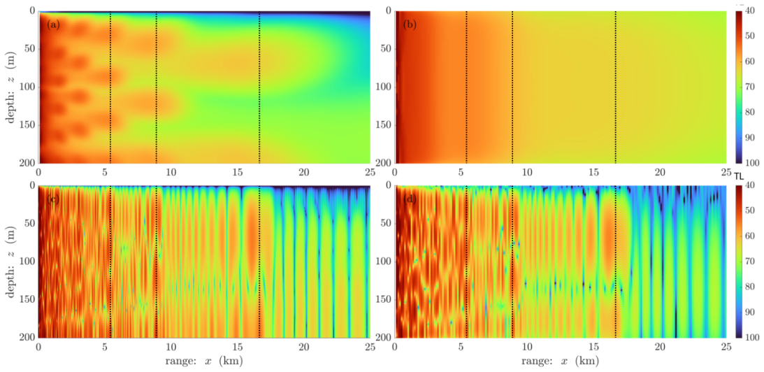
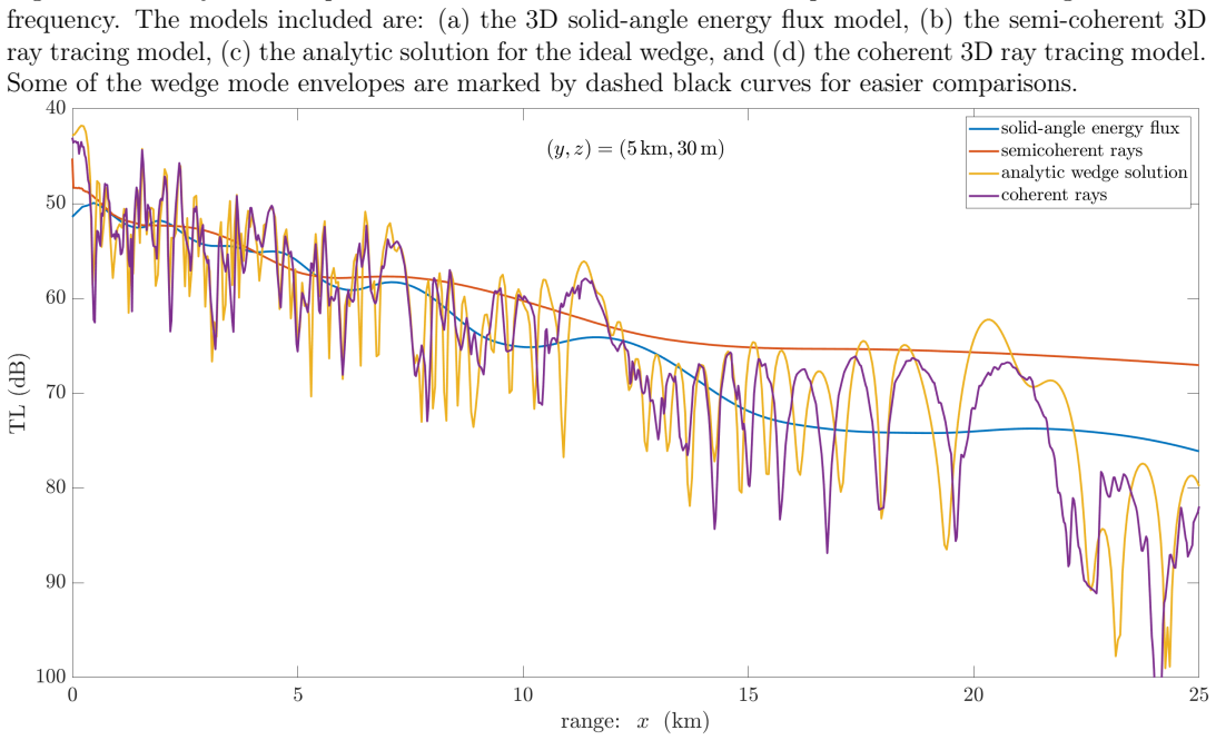
- [Section III.C-D, Figs. 5-16] The validation is entirely qualitative: no error norms, mean/median absolute TL errors, or correlation metrics are reported for any of the comparisons against analytic, PE, or ray solutions. The paper itself concedes a 'TL offset, approximately 10 dB at 25 km range' in Figs. 6 and 8. Since the abstract and Section III claim that fields 'compare favorably,' the absence of quantitative metrics makes this the central supporting evidence insufficient. Please add range/depth-averaged error metrics for the line-array comparisons and, where appropriate, spatial error maps for the 2D slices.
- [Section II.G, eqs. (89)-(93), and Section III.C] The convergence factor depends on the maximum mode-number differences δ⊤_m and δ⊤_n through F_m = 1 + 2δ⊤_m and F_n = 1 + 2δ⊤_n, and Section III.C states that δ⊤_n 'affects the size and shape of the focused intensity lobes.' Yet the values of δ⊤_m and δ⊤_n used for Figs. 5-16 are never reported. Without these values and a sensitivity study, it is impossible to determine whether the lobe agreement with the analytic wedge solution is a predictive test of the model's physics or a consequence of tuned focusing parameters. Please report the parameter values and demonstrate robustness across a reasonable range.
- [Section III.D, Figs. 11-16] The lossy penetrable wedge results contain a 'noticeable horizontal intensity band or caustic-like effect' that the text describes as 'likely an artifact' whose 'exact cause is currently unknown.' This artifact appears in the benchmark environment used to support the model's central claim, and it is not confined to a peripheral plot. The manuscript needs either to explain and remove the artifact, or to quantify its spatial extent and show that it does not compromise the claimed agreement with the PE reference solution in the regions used for validation.
- [Section II.A and Section V] The model's derivation assumes the environment is translationally symmetric along the forward x-axis, which eliminates back-propagation and makes the forward wavenumber k_xmn constant. This is a strong restriction: it excludes along-axis geological or oceanographic variability, so the model is not a general 3D solver. The abstract's phrase '3D ocean acoustic environments' and Section V's 'generalized 3D waveguides' overstate the scope. Please either qualify the claims explicitly to 'transversely range-dependent, longitudinally invariant' environments, or implement and validate the forward adiabatic x-range-dependence that Section IV only discusses as future work.
- [Abstract and Section III.A] The abstract claims that the required computational effort is 'predominantly independent of range and frequency,' but the manuscript provides no runtime measurements, scaling experiments, or complexity analysis to support this. The implementation section describes vectorization and parallelization but not how the cost varies with range, frequency, or receiver count. Please include at least a scaling benchmark that varies frequency and range, with wall-clock times, to substantiate the efficiency claim.
minor comments (4)
- [Section II.F] There is a typo in 'the averge acoustic energy density'; it should read 'average.'
- [Equations (71) and (74)] The WKB limiter in Eq. (71) and the elevation-angle floor in Eq. (74) introduce heuristic or user-set elements. Please clarify how the constants in the limiter are chosen and report the exact |θ|^⊥, |θ|^⊤, and ε_ϕ values used for each figure, since these affect the computed TL fields.
- [Figures 5, 7, 9, 11, 13, 15] The side-by-side 2D TL panels would be much more informative if they used a shared color scale and colorbars; without colorbars the reader cannot compare intensity levels across models.
- [Section III.A] The implementation relies on Matlab's contour-search routines for the adiabatic invariance mapping; a brief statement about the grid resolution and convergence of that search would help reproducibility.
Circularity Check
No significant circularity: the TL field is a forward Helmholtz-derived integral checked against independent analytic, PE, and ray solutions; the unreported δ⊤_n and ~10 dB offset are validation/transparency gaps, not construction equivalences.
full rationale
The model's field expression (eq. 127) is built from a double mode-sum cross-product of the 3D Helmholtz Green's function (eqs. 19–24), transformed to a solid-angle integral via the closed-phase Jacobian (eqs. 62–64), with kernels for convergence, mode-stripping, bottom attenuation, and directivity derived from wavenumber cycle integrals. No fitted parameter enters the definition of P; the environment and source/receiver geometry determine the field. The Section III comparisons are against external references: the analytic ideal-wedge solution of Buckingham/Frisk, Bellhop3D ray tracing, and Lin's 3D wide-angle split-step PE model. The energy-flux TL is not constructed from those outputs, so the central 'captures horizontal refraction' claim is not circular. Ref. [1] (Langhirt's prior work) is cited for components such as the mode-stripping kernel and trajectory inversion, but those mechanisms are re-derived in Sections II.G–II.M, so the self-citation is supporting rather than load-bearing. The unreported convergence-factor widths δ⊤_m/δ⊤_n (eqs. 89–93) affect lobe size and shape and are a transparency/reproducibility gap; yet the paper does not state that they were fitted to the analytic solution, and lobe positions are set by the Ξm/Ξn phase arguments from wavenumber integrals, so no reduction-to-fit can be exhibited. The admitted ~10 dB offset and the unexplained horizontal intensity band are correctness/validation concerns, not circularity. Overall the derivation is self-contained and externally benchmarked.
Assumptions & free parameters
free parameters (3)
- F_m, F_n (convergence factor widths) =
not reported
- Finite-frequency elevation angle floor |θ|^⊥ =
asin(c0/(4 f H0))
- Azimuthal epsilon buffer ε_φ =
not specified
assumptions (5)
- domain assumption Adiabatic approximation: vertical modenumbers are invariant and vertical modes decouple from range dependence
- domain assumption Environment is translationally invariant along the forward x-axis with no back-propagation
- domain assumption All wavenumber profiles are convex and transverse variability is mild enough to neglect non-convex effective profiles
- domain assumption WKB approximation and modal continuum (high-frequency limit)
- domain assumption Bottom attenuation described by a local grazing-angle-dependent plane-wave reflection coefficient
Cite this review
Pith. "Pith review of A three-dimensional energy flux acoustic propagation model." pith.science (2026). https://pith.science/paper/PXOA3OXA
@misc{pith2026250603325,
  author       = {Pith},
  title        = {Pith review of: A three-dimensional energy flux acoustic propagation model},
  year         = {2026},
  howpublished = {\url{https://pith.science/paper/PXOA3OXA}},
  note         = {Machine review of arXiv:2506.03325}
}
read the original abstract
This paper extends energy flux methods to handle three-dimensional ocean acoustic environments, the implemented solution captures horizontally refracted incoherent acoustic intensity, and its required computational effort is predominantly independent of range and frequency. Energy flux models are principally derived as incoherent solutions for acoustic propagation in bounded waveguides. The angular distribution of incoherent acoustic intensity may be derived from Wentzel-Kramers-Brillouin modes transformed to the continuous angular domain via the ray-mode analogy. The adiabatic approximation maps angular distributions of acoustic intensity as waveguide properties vary along a range-dependent environment, and the final solution integrates a modal intensity kernel over propagation angles. Additional integration kernels can be derived that modulate the incoherent field by specific physical wave phenomena such as geometric spreading, refractive focusing, and boundary attenuation and interference. This three-dimensional energy flux model is derived from a double-mode-sum cross-product, is integrated over solid-angles, incorporates a bi-variate convergence factor, accounts for acoustic energy escaping the computational domain through transparent transverse boundaries, and accumulates bottom attenuation along transverse cycle trajectories. Transmission loss fields compare favorably with analytic, ray tracing, and parabolic equation solutions for the canonical ASA wedge problem, and three-dimensional adiabatic ray trajectories for the ideal wedge are demonstrated.
Figures


Figures from the paper (15 more)





Reference graph
Works this paper leans on
-
[1]
Foundations for Development of Three-Dimensional Energy Flux Acoustic Propa- gation Models
Mark Langhirt. “Foundations for Development of Three-Dimensional Energy Flux Acoustic Propa- gation Models”. In: (2025)
work page 2025
-
[2]
Guided propagation in a slowly varying medium
DE Weston. “Guided propagation in a slowly varying medium”. In:Proceedings of the Physical Society 73.3 (1959), p. 365
work page 1959
-
[3]
Averagefieldinanunderwatersoundchannel
LMBrekhovskikh.“Averagefieldinanunderwatersoundchannel”.In: SOVIET PHYSICS ACOUSTICS- USSR 11.2 (1965), pp. 126–+
work page 1965
-
[4]
Ray and wave invariants for SOFAR channel propagation
D Michael Milder. “Ray and wave invariants for SOFAR channel propagation”. In:The Journal of the Acoustical Society of America46.5B (1969), pp. 1259–1263
work page 1969
-
[5]
Acoustic flux formulas for range-dependent ocean ducts
DE Weston. “Acoustic flux formulas for range-dependent ocean ducts”. In:The Journal of the Acous- tical Society of America68.1 (1980), pp. 269–281
work page 1980
-
[6]
Acoustic flux methods for oceanic guided waves
DE Weston. “Acoustic flux methods for oceanic guided waves”. In: The Journal of the Acoustical Society of America68.1 (1980), pp. 287–296. 51
work page 1980
-
[7]
Wave-theory peaks in range-averaged channels of uniform sound velocity
DE Weston. “Wave-theory peaks in range-averaged channels of uniform sound velocity”. In: The Journal of the Acoustical Society of America68.1 (1980), pp. 282–286
work page 1980
-
[8]
The equivalence of bottom loss and mode attenuation per cycle in underwater acoustics
CT Tindle. “The equivalence of bottom loss and mode attenuation per cycle in underwater acoustics”. In: The Journal of the Acoustical Society of America66.1 (1979), pp. 250–255
work page 1979
Show all 35 references
-
[9]
Reflection loss and mode attenuation in a Pekeris model
DE Weston and CT Tindle. “Reflection loss and mode attenuation in a Pekeris model”. In: The Journal of the Acoustical Society of America66.3 (1979), pp. 872–879
1979
-
[10]
Connection of acoustic beam displacement, cycle dis- tances, and attenuations for rays and normal modes
Christopher T Tindle and David E Weston. “Connection of acoustic beam displacement, cycle dis- tances, and attenuations for rays and normal modes”. In:The Journal of the Acoustical Society of America 67.5 (1980), pp. 1614–1622
1980
-
[11]
Cycle distances and attenuation in shallow water
CT Tindle, DE Weston, and SG Payne. “Cycle distances and attenuation in shallow water”. In:The Journal of the Acoustical Society of America68.5 (1980), pp. 1489–1492
1980
-
[12]
Horizontal refraction in a three-dimensional medium of variable stratification
DE Weston. “Horizontal refraction in a three-dimensional medium of variable stratification”. In: Proceedings of the Physical Society78.1 (1961), p. 46
1961
-
[13]
Three-dimensional ray paths in basins, troughs, and near seamounts by use of ray invariants
Chris H Harrison. “Three-dimensional ray paths in basins, troughs, and near seamounts by use of ray invariants”. In:The journal of the acoustical society of America62.6 (1977), pp. 1382–1388
1977
-
[14]
Acoustic shadow zones in the horizontal plane
Chris H Harrison. “Acoustic shadow zones in the horizontal plane”. In:The Journal of the Acoustical Society of America65.1 (1979), pp. 56–61
1979
-
[15]
Ray convergence in a flux-like propagation formulation
Chris H Harrison. “Ray convergence in a flux-like propagation formulation”. In:The Journal of the Acoustical Society of America133.6 (2013), pp. 3777–3789
2013
-
[16]
Efficient modeling of range-dependent ray convergence effects in propagation and reverberation
Chris H Harrison. “Efficient modeling of range-dependent ray convergence effects in propagation and reverberation”. In:The Journal of the Acoustical Society of America137.5 (2015), pp. 2982–2985
2015
-
[17]
George B Arfken and Hans J Weber.Mathematical methods for physicists. 1999
1999
-
[18]
Applied partial differential equations with Fourier series and boundary value problems
Richard Haberman. Applied partial differential equations with Fourier series and boundary value problems. Pearson Higher Ed, 2012
2012
-
[19]
Methods of theoretical physics
Philip M Morse and Herman Feshbach. “Methods of theoretical physics”. In:American Journal of Physics 22.6 (1954), pp. 410–413
1954
-
[20]
Fundamentals of ocean acoustics
Leonid Maksimovich Brekhovskikh, Yu P Lysanov, and Jurij P Lysanov. Fundamentals of ocean acoustics. Springer Science & Business Media, 2003. 52
2003
-
[21]
Carl M Bender and Steven A Orszag.Advanced mathematical methods for scientists and engineers I: Asymptotic methods and perturbation theory. Vol. 1. Springer Science & Business Media, 1999
1999
-
[22]
Averaged sound transmission in range-dependent channels
Preston W Smith. “Averaged sound transmission in range-dependent channels”. In:The Journal of the Acoustical Society of America55.6 (1974), pp. 1197–1204
1974
-
[23]
Integrating the energy flux method for reverberation with physics-based seabed scattering models: Modeling and inversion
Ji-Xun Zhou and Xue-Zhen Zhang. “Integrating the energy flux method for reverberation with physics-based seabed scattering models: Modeling and inversion”. In:The Journal of the Acousti- cal Society of America134.1 (2013), pp. 55–66
2013
-
[24]
Finn B Jensen et al.Computational ocean acoustics. Vol. 2011. Springer, 2011
2011
-
[25]
Acoustics of layered media I: Plane and quasi-plane waves
Leonid M Brekhovskikh and Oleg A Godin. Acoustics of layered media I: Plane and quasi-plane waves. Vol. 5. Springer Science & Business Media, 2012
2012
-
[26]
Leonid M Brekhovskikh and Oleg A Godin.Acoustics of layered media II: Point sources and bounded beams. Vol. 10. Springer Science & Business Media, 2013
2013
-
[27]
Acoustics: an introduction to its physical principles and applications
Allan D Pierce. Acoustics: an introduction to its physical principles and applications. Springer, 2019
2019
-
[28]
Propagation in a waveguide with range-dependent seabed properties
Charles W Holland. “Propagation in a waveguide with range-dependent seabed properties”. In:The Journal of the Acoustical Society of America128.5 (2010), pp. 2596–2609
2010
-
[29]
The bellhop manual and user’s guide: Preliminary draft
Michael B Porter. “The bellhop manual and user’s guide: Preliminary draft”. In:Heat, Light, and Sound Research, Inc., La Jolla, CA, USA, Tech. Rep260 (2011)
2011
-
[30]
Mark Adam Langhirt. Tethys. Version 1.0.0. May 2025.url: https://github.com/marklanghirt/ Tethys
2025
-
[31]
Numerical solutions of range-dependent benchmark problems in ocean acoustics
Finn B Jensen and Carlo M Ferla. “Numerical solutions of range-dependent benchmark problems in ocean acoustics”. In:The Journal of the Acoustical Society of America87.4 (1990), pp. 1499–1510
1990
-
[32]
Acoustic propagation in a wedge-shaped ocean with perfectly reflecting bound- aries
M J Buckingham. “Acoustic propagation in a wedge-shaped ocean with perfectly reflecting bound- aries”. In: NATO Advanced Research Workshop on Hybrid Formulation of Wave Propagation and Scattering (Castel Gandolfo, Italy, Aug. 30, 1983). Ed. by L B Felsen. Vol. 86. NATO ASI Ser...
1983
-
[33]
Acoustic propagation in a wedge-shaped ocean with perfectly reflecting boundaries
Michael J Buckingham. “Acoustic propagation in a wedge-shaped ocean with perfectly reflecting boundaries”. In:Hybrid formulation of wave propagation and scattering. Dordrecht: Martinus Nijhoff Publishers, 1984, pp. 77–99. 53
1984
-
[34]
Ocean and seabed acoustics: a theory of wave propagation
George V Frisk. Ocean and seabed acoustics: a theory of wave propagation. Pearson Education, 1994
1994
-
[35]
A higher-order tangent linear parabolic-equation solution of three-dimensional sound propagation
Ying-Tsong Lin. “A higher-order tangent linear parabolic-equation solution of three-dimensional sound propagation”. In: The Journal of the Acoustical Society of America134.2 (2013), EL251– EL257. 54
2013
Reviewed August 7, 2026 · model on record in the stance chip above.
Discussion (0). Sign in to comment.