REVIEW 5 minor 97 references
Integrating Background Knowledge for Scalable Causal Discovery
T0 review · 0 major / 5 minor · reviewed 2026-07-14 · grok-4.5
Pith's one-line read Background knowledge used during causal discovery can cut CI tests by an order of magnitude while improving effect estimates.
desk verdict Solid engineering paper: careful during-search BK (especially delayed gap handling) for PC/SNAP/local methods, with proofs and clear CI/runtime gains under consistent BK. read the letter →
The pith
A machine-rendered reading of the paper's core claim, the machinery that carries it, and where it could break.
The reading
What carries the argument
The three operating principles (skip known adjacencies, restrict separators to possible parents given the current skeleton and BK, and search for separators of known gaps only after the first skeleton pass) together with the b-possible-ancestral pruning rule that lets SNAP keep only the variables still needed for the targets.
What would settle it
Run the same suite of algorithms on graphs with deliberately injected BK errors (as in the paper’s own App. J) and check whether the claimed reductions in CI-test count and intervention distance still appear once the error rate exceeds roughly 10–20 percent.
Extended reading notes
Core claim
When background knowledge about direct causal relations is used inside the discovery loop—skipping known adjacencies, restricting candidate separators to possible parents, and delaying gap tests until the skeleton is sparse—the resulting algorithms recover the same (or a correctly restricted) MPDAG or local structure while performing substantially fewer conditional-independence tests.
Load-bearing premise
The supplied background knowledge never contradicts the true causal graph; if it does, edges may be kept or mis-oriented and some algorithms become slower rather than faster.
Editorial analysis
A structured set of objections, weighed in public.
Referee Report
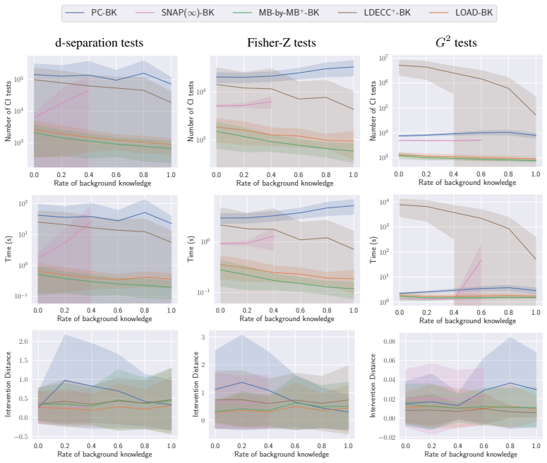
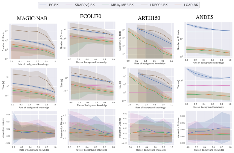
Summary. The paper develops a framework for integrating background knowledge (BK) about direct causal relations (adjacencies, orientations, and gaps) into the causal discovery process itself, rather than only as post-processing. It focuses on scalable methods that recover only relevant subgraphs or local structure. The authors instantiate the framework for PC, SNAP(k)/SNAP(∞), MB-by-MB, LDECC, LOAD, and two Markov-blanket algorithms (Grow-Shrink, Total Conditioning). Core design choices include skipping CI tests for known adjacencies, restricting candidate separators to possible parents under BK, and delaying (rather than naively removing) known gaps so that separating sets remain well-defined for v-structure orientation. Under oracle CI tests and consistent BK they prove soundness for all variants and completeness for all except LDECC-BK (Thms. 3.1–3.4, Cor. 3.1–3.2, App. C). Experiments on Erdős–Rényi graphs and bnlearn networks show reductions in CI tests and runtime, with improved or preserved intervention distance as the BK rate rises (Fig. 1, Apps. G–K), plus ablations on BK type, imperfect BK, and post-processing baselines.
Significance. The work addresses a genuine practical bottleneck: constraint-based discovery becomes expensive at scale, yet expert or experimental BK is often available and currently under-used during search. The technical contribution is concrete and reusable—shared subroutines (SkelStep-BK, MissingSepsets-BK, PossPa, PossMB) plus algorithm-specific adaptations that avoid known failure modes of library implementations (App. D). Soundness/completeness proofs with counter-examples for incorrect designs (Ex. C.1–C.4), reproducible code, and multi-metric evaluation (CI counts, time, intervention distance, SHD for global methods) strengthen the claim. The imperfect-BK ablations (App. J) and post-processing comparisons (App. H) make the scope of the claims transparent. If the results hold, the framework is immediately useful for practitioners who already run PC/SNAP/local methods and have partial edge knowledge.
minor comments (5)
- In Sec. 3.1 the definition of PossPa_G(X,B) is given inline; a numbered equation would make later references (e.g., the adjusted PossPa* in Eq. (1) for MB-by-MB) cleaner.
- Fig. 1 packs five algorithms × three data regimes; the caption and legend are dense. A short table of relative CI-test reductions at BK rate 0.5 would help readers extract the main quantitative message.
- App. E.2 (FCI-BK) is preliminary and correctly labeled as such; a one-sentence pointer in the main conclusions that latent-variable completeness remains open would set expectations more clearly for readers who skip the appendix.
- A few typos: “SkelStep-BK” vs “SkelStep” consistency in Alg. 4 line 5; “WaiList” in Ex. C.3; “or all CI tests” (missing “f”) in Sec. 5.
- Related work could briefly note how the delayed-gap strategy differs from fixedGaps in pcalg/causal-learn/pgmpy (already illustrated in App. D) so that the novelty relative to existing library options is explicit in the main text.
Circularity Check
No significant circularity: algorithmic soundness under stated assumptions plus empirical comparisons; no fitted inputs re-labeled as predictions.
full rationale
The paper's central claims are (i) soundness/completeness theorems for BK-aware variants of PC, SNAP, MB-by-MB, LOAD, and GrowShrink under oracle CI tests and consistent background knowledge B, and (ii) empirical reductions in CI tests/runtime with non-worsening intervention distance as the BK rate rises. The theorems are proved by adapting standard PC/RFCI/Meek arguments and prior SNAP/LOAD lemmas (App. C); they do not define the target MPDAG or local structure in terms of the algorithm's own output. Empirical intervention distance is measured on held-out samples of size 10000, not on quantities fitted from the discovery data. Self-citations to SNAP and LOAD are prior methods being extended with BK subroutines (SkelStep-BK, MissingSepsets-BK, PossPa), not uniqueness theorems or ansätze that force the new results. Gap-handling is motivated by concrete library failures (App. D) and covered by the soundness proofs rather than by redefining non-adjacency. Imperfect-BK ablations (App. J) are reported as degradation, not as predictions. No step reduces a claimed prediction or first-principles result to its inputs by construction. Score 0 is therefore appropriate.
Assumptions & free parameters
free parameters (4)
- CI significance level α =
0.01
- BK sampling rate and type mix =
0–1 rate; uniform adj/orient when adjacent
- Erdős–Rényi graph ensemble =
n=100, E[deg]=3, maxdeg=10
- Imperfect-BK error rates =
10% adj/orient, 5% gaps (main imperfect); 0–30% sweep
assumptions (5)
- domain assumption Observational distribution p is Markov and faithful to the true causal DAG D.
- domain assumption No latent confounders or selection bias in the main contributions.
- domain assumption Background knowledge B is consistent with the true DAG D.
- standard math If X and Y are non-adjacent then they are d-separated by Pa(X) or Pa(Y) (Spirtes et al. Lem. 3.3.9).
- standard math Meek orientation rules and MPDAG theory of Perković et al. correctly maximize orientations given BK.
Cite this review
Pith. "Pith review of Integrating Background Knowledge for Scalable Causal Discovery." pith.science (2026). https://pith.science/paper/PZIZMA3L
@misc{pith2026260710456,
  author       = {Pith},
  title        = {Pith review of: Integrating Background Knowledge for Scalable Causal Discovery},
  year         = {2026},
  howpublished = {\url{https://pith.science/paper/PZIZMA3L}},
  note         = {Machine review of arXiv:2607.10456}
}
read the original abstract
Expert background knowledge is often available in practical applications of causal discovery. Such constraints on the true causal graph can help causal discovery in terms of identifiability of causal effects and accuracy of the learned structure, but also in reducing the space of candidate causal graphs. As causal discovery can become computationally expensive for large number of variables, it is crucial to utilize background knowledge effectively during the causal discovery process. However, most current methods only use background knowledge in a postprocessing step after causal discovery to refine the learned graph. In this work, we develop a framework for utilizing background knowledge during the causal discovery process, focusing especially on scalable causal discovery methods that recover only a subset of the whole graph. We implement our framework for multiple algorithms and empirically show that utilizing background knowledge can both reduce computational requirements and increase the quality of the learned structures.
Figures


Figures from the paper (13 more)



Reference graph
Works this paper leans on
-
[1]
Cambridge university press, 2009
Judea Pearl.Causality. Cambridge university press, 2009
2009
-
[2]
Review of causal discovery methods based on graphical models.Frontiers in Genetics, 10, 2019
Clark Glymour, Kun Zhang, and Peter Spirtes. Review of causal discovery methods based on graphical models.Frontiers in Genetics, 10, 2019. ISSN 1664-8021. doi: 10.3389/fgene.2019. 00524
-
[3]
Maathuis
Emilija Perkovi´c, Johannes Textor, Markus Kalisch, and Marloes H. Maathuis. Complete graphical characterization and construction of adjustment sets in markov equivalence classes of ancestral graphs.Journal of Machine Learning Research, 18(220):1–62, 2018. URL http://jmlr.org/papers/v18/16-319.html
2018
-
[4]
Inferring causation from time series in earth system sciences.Nature communications, 10(1):2553, 2019
Jakob Runge, Sebastian Bathiany, Erik Bollt, Gustau Camps-Valls, Dim Coumou, Ethan Deyle, Clark Glymour, Marlene Kretschmer, Miguel D Mahecha, Jordi Mu˜noz-Mar´ı, et al. Inferring causation from time series in earth system sciences.Nature communications, 10(1):2553, 2019
2019
-
[5]
Jacqueline Maasch, Kyra Gan, Violet Chen, Agni Orfanoudaki, Nil-Jana Akpinar, and Fei Wang. Local causal discovery for structural evidence of direct discrimination.Proceedings of the AAAI Conference on Artificial Intelligence, 39(18):19349–19357, Apr. 2025. doi: 10.1609/aaai. v39i18.34130. URLhttps://ojs.aaai.org/index.php/AAAI/article/view/34130
doi:10.1609/aaai 2025
-
[6]
Causal discovery under a confounder blanket
David S Watson and Ricardo Silva. Causal discovery under a confounder blanket. InUncertainty in Artificial Intelligence, pages 2096–2106. PMLR, 2022
-
[7]
Jacqueline R. M. A. Maasch, Weishen Pan, Shantanu Gupta, V olodymyr Kuleshov, Kyra Gan, and Fei Wang. Local discovery by partitioning: Polynomial-time causal discovery around exposure-outcome pairs. InThe 40th Conference on Uncertainty in Artificial Intelligence, 2024
2024
-
[8]
Snap: Sequential non-ancestor pruning for targeted causal effect estimation with an unknown graph
M´aty´as Schubert, Tom Claassen, and Sara Magliacane. Snap: Sequential non-ancestor pruning for targeted causal effect estimation with an unknown graph. In Yingzhen Li, Stephan Mandt, Shipra Agrawal, and Emtiyaz Khan, editors,Proceedings of The 28th International Conference on Artificial Intelligence and Statistics, volume 258 ofProceedings of Machine Lea...
2025
Show all 97 references
-
[9]
Discovering and orienting the edges connected to a target variable in a dag via a sequential local learning approach.Computational statistics & data analysis, 77:252–266, 2014
Changzhang Wang, You Zhou, Qiang Zhao, and Zhi Geng. Discovering and orienting the edges connected to a target variable in a dag via a sequential local learning approach.Computational statistics & data analysis, 77:252–266, 2014
2014
-
[10]
Local causal discovery for estimating causal effects
Shantanu Gupta, David Childers, and Zachary Chase Lipton. Local causal discovery for estimating causal effects. InConference on Causal Learning and Reasoning, pages 408–447. PMLR, 2023
2023
-
[11]
Local causal discovery for statistically efficient causal inference
M´aty´as Schubert, Tom Claassen, and Sara Magliacane. Local causal discovery for statistically efficient causal inference. InThe 29th International Conference on Artificial Intelligence and Statistics, 2026. URLhttps://openreview.net/forum?id=FlWl20PFd7
2026
-
[12]
Maathuis
Emilija Perkovi´c, Markus Kalisch, and Marloes H. Maathuis. Interpreting and using cpdags with background knowledge. In Gal Elidan, Kristian Kersting, and Alexander Ihler, editors, Proceedings of the Thirty-Third Conference on Uncertainty in Artificial Intelligence, UAI 2017, ...
2017
-
[13]
On the representation of pairwise causal background knowledge and its applications in causal inference.Journal of Machine Learning Research, 26(229):1–73, 2025
Zhuangyan Fang, Ruiqi Zhao, Yue Liu, and Yangbo He. On the representation of pairwise causal background knowledge and its applications in causal inference.Journal of Machine Learning Research, 26(229):1–73, 2025. URLhttp://jmlr.org/papers/v26/23-0624.html
2025
-
[14]
Do we become wiser with time? on causal equivalence with tiered background knowledge
Christine W Bang and Vanessa Didelez. Do we become wiser with time? on causal equivalence with tiered background knowledge. InUncertainty in Artificial Intelligence, pages 119–129. PMLR, 2023
2023
-
[15]
Ancestral causal inference.Advances in Neural Information Processing Systems, 29, 2016
Sara Magliacane, Tom Claassen, and Joris M Mooij. Ancestral causal inference.Advances in Neural Information Processing Systems, 29, 2016. 10
2016
-
[16]
Sample efficient active learning of causal trees
Kristjan Greenewald, Dmitriy Katz, Karthikeyan Shanmugam, Sara Magliacane, Murat Ko- caoglu, Enric Boix Adsera, and Guy Bresler. Sample efficient active learning of causal trees. In H. Wallach, H. Larochelle, A. Beygelzimer, F. d'Alch ´e-Buc, E. Fox, and R. Garnett, ed- itors,...
2019
-
[17]
Large language models for causal discovery: Current landscape and future directions
Guangya Wan, Yunsheng Lu, Yuqi Wu, Mengxuan Hu, and Sheng Li. Large language models for causal discovery: Current landscape and future directions. In James Kwok, editor,Proceedings of the Thirty-Fourth International Joint Conference on Artificial Intelligence, IJCAI-25, pages ...
2025 doi
-
[18]
On the reliability of large language models for causal discovery
Tao Feng, Lizhen Qu, Niket Tandon, Zhuang Li, Xiaoxi Kang, and Gholamreza Haffari. On the reliability of large language models for causal discovery. InProceedings of the 63rd Annual Meeting of the Association for Computational Linguistics (Volume 1: Long Papers), pages 9565–9590, 2025
2025
-
[19]
Prior-knowledge-driven local causal structure learning and its application on causal discovery between type 2 diabetes and bone mineral density.IEEE Access, 8:108798–108810,
Wei Wang, Gangqiang Hu, Bo Yuan, Shandong Ye, Chao Chen, Yayun Cui, Xi Zhang, and Liting Qian. Prior-knowledge-driven local causal structure learning and its application on causal discovery between type 2 diabetes and bone mineral density.IEEE Access, 8:108798–108810,
-
[20]
doi: 10.1109/ACCESS.2020.2994936
2020 doi
-
[21]
Challenges and opportunities with causal discovery algorithms: application to alzheimer’s pathophysiology.Scientific reports, 10(1):2975, 2020
Xinpeng Shen, Sisi Ma, Prashanthi Vemuri, and Gyorgy Simon. Challenges and opportunities with causal discovery algorithms: application to alzheimer’s pathophysiology.Scientific reports, 10(1):2975, 2020
2020
-
[22]
Reisch, D ´enes Moln´ar, Stefaan De Henauw, Luis Moreno, Toomas Veidebaum, Michael Tornaritis, Iris Pigeot, and Vanessa Didelez
Ronja Foraita, Janine Witte, Claudia B¨ornhorst, Wencke Gwozdz, Valeria Pala, Lauren Lissner, Fabio Lauria, Lucia A. Reisch, D ´enes Moln´ar, Stefaan De Henauw, Luis Moreno, Toomas Veidebaum, Michael Tornaritis, Iris Pigeot, and Vanessa Didelez. A longitudinal causal graph ana...
2024 doi
-
[23]
Constraint-based causal discovery: Conflict resolution with answer set programming
Antti Hyttinen, Frederick Eberhardt, and Matti J¨arvisalo. Constraint-based causal discovery: Conflict resolution with answer set programming. In Jin Tian and {Nevin L.} Zhang, editors, Proceedings of the 30th Conference on Uncertainty in Artificial Intelligence (UAI 2014), pa...
2014
-
[24]
Constraint-based causal discovery from multiple interventions over overlapping variable sets.Journal of Machine Learning Research, 16(66): 2147–2205, 2015
Sofia Triantafillou and Ioannis Tsamardinos. Constraint-based causal discovery from multiple interventions over overlapping variable sets.Journal of Machine Learning Research, 16(66): 2147–2205, 2015. URLhttp://jmlr.org/papers/v16/triantafillou15a.html
2015
-
[25]
Mooij, Sara Magliacane, and Tom Claassen
Joris M. Mooij, Sara Magliacane, and Tom Claassen. Joint causal inference from multiple contexts.Journal of Machine Learning Research, 21(99):1–108, 2020. URL http://jmlr. org/papers/v21/17-123.html
2020
-
[26]
MIT Press, 2nd edition, 2000
Peter Spirtes, Clark Glymour, and Richard Scheines.Causation, Prediction, and Search. MIT Press, 2nd edition, 2000
2000
-
[27]
Causal inference and causal explanation with background knowledge
Christopher Meek. Causal inference and causal explanation with background knowledge. In Proceedings of the Eleventh Conference on Uncertainty in Artificial Intelligence, UAI’95, page 403–410, San Francisco, CA, USA, 1995. Morgan Kaufmann Publishers Inc. ISBN 1558603859
1995
-
[28]
Maathuis, and Peter B¨uhlmann
Markus Kalisch, Martin M¨achler, Diego Colombo, Marloes H. Maathuis, and Peter B¨uhlmann. Causal inference using graphical models with the R package pcalg.Journal of Statistical Software, 47(11):1–26, 2012. doi: 10.18637/jss.v047.i11
2012 doi
-
[29]
Causal-learn: Causal discovery in python.Journal of Machine Learning Research, 25(60):1–8, 2024
Yujia Zheng, Biwei Huang, Wei Chen, Joseph Ramsey, Mingming Gong, Ruichu Cai, Shohei Shimizu, Peter Spirtes, and Kun Zhang. Causal-learn: Causal discovery in python.Journal of Machine Learning Research, 25(60):1–8, 2024. 11
2024
-
[30]
Tetrad—a toolbox for causal discovery.8th international workshop on climate informatics, 2018
Joseph D Ramsey, Kun Zhang, Madelyn Glymour, Ruben Sanchez Romero, Biwei Huang, Imme Ebert-Uphoff, Savini Samarasinghe, Elizabeth A Barnes, and Clark Glymour. Tetrad—a toolbox for causal discovery.8th international workshop on climate informatics, 2018
2018
-
[31]
pgmpy: A python toolkit for bayesian networks.Journal of Machine Learning Research, 25(265):1–8, 2024
Ankur Ankan and Johannes Textor. pgmpy: A python toolkit for bayesian networks.Journal of Machine Learning Research, 25(265):1–8, 2024. URL http://jmlr.org/papers/v25/ 23-0487.html
2024
-
[32]
Learning high-dimensional directed acyclic graphs with latent and selection variables.The Annals of Statistics, pages 294–321, 2012
Diego Colombo, Marloes H Maathuis, Markus Kalisch, and Thomas S Richardson. Learning high-dimensional directed acyclic graphs with latent and selection variables.The Annals of Statistics, pages 294–321, 2012
2012
-
[33]
Bayesian network induction via local neighborhoods
Dimitris Margaritis and Sebastian Thrun. Bayesian network induction via local neighborhoods. Advances in neural information processing systems, 12, 1999
1999
-
[34]
Using markov blankets for causal structure learning
Jean-Philippe Pellet and Andr´e Elisseeff. Using markov blankets for causal structure learning. Journal of Machine Learning Research, 9(7), 2008
2008
-
[35]
Local Causal Discovery with Background Knowledge .IEEE Transactions on Pattern Analysis & Machine Intelligence, pages 1– 12, February 2026
Qingyuan Zheng, Yue Liu, and Yangbo He. Local Causal Discovery with Background Knowledge .IEEE Transactions on Pattern Analysis & Machine Intelligence, pages 1– 12, February 2026. ISSN 1939-3539. doi: 10.1109/TPAMI.2026.3667409. URL https: //doi.ieeecomputersociety.org/10.1109...
2026 doi
-
[36]
Improving finite sample performance of causal discovery by exploiting temporal structure.arXiv preprint arXiv:2406.19503, 2024
Christine W Bang, Janine Witte, Ronja Foraita, and Vanessa Didelez. Improving finite sample performance of causal discovery by exploiting temporal structure.arXiv preprint arXiv:2406.19503, 2024
2024 arXiv
-
[37]
Bryan Andrews, Peter Spirtes, and Gregory F. Cooper. On the completeness of causal discovery in the presence of latent confounding with tiered background knowledge. In Silvia Chiappa and Roberto Calandra, editors,Proceedings of the Twenty Third International Conference on Arti...
2020
-
[38]
Constraint-based causal discovery with tiered back- ground knowledge and latent variables in single or overlapping datasets.Proceedings of Machine Learning Research, 275:1–31, 2025
Christine W Bang and Vanessa Didelez. Constraint-based causal discovery with tiered back- ground knowledge and latent variables in single or overlapping datasets.Proceedings of Machine Learning Research, 275:1–31, 2025
2025
-
[39]
Score-based causal discovery with temporal background information.arXiv preprint arXiv:2502.06232, 2025
Tobias Ellegaard Larsen, Claus Thorn Ekstrøm, and Anne Helby Petersen. Score-based causal discovery with temporal background information.arXiv preprint arXiv:2502.06232, 2025
2025 arXiv
-
[40]
Sound and complete causal identification with latent variables given local background knowledge.Artificial Intelligence, 322:103964,
Tian-Zuo Wang, Tian Qin, and Zhi-Hua Zhou. Sound and complete causal identification with latent variables given local background knowledge.Artificial Intelligence, 322:103964,
-
[41]
doi: https://doi.org/10.1016/j.artint.2023.103964
ISSN 0004-3702. doi: https://doi.org/10.1016/j.artint.2023.103964. URL https: //www.sciencedirect.com/science/article/pii/S0004370223001108
2023 doi
-
[42]
Towards complete causal explanation with expert knowledge.arXiv preprint arXiv:2407.07338, 2024
Aparajithan Venkateswaran and Emilija Perkovi´c. Towards complete causal explanation with expert knowledge.arXiv preprint arXiv:2407.07338, 2024
2024 arXiv
-
[43]
A logical characterization of constraint-based causal discovery
Tom Claassen and Tom Heskes. A logical characterization of constraint-based causal discovery. InProceedings of the Twenty-Seventh Conference on Uncertainty in Artificial Intelligence, pages 135–144, 2011
2011
-
[44]
A hybrid algorithm for learning causal networks using uncertain experts’ knowledge
Christophe Gonzales, Axel Journe, and Ahmed Mabrouk. A hybrid algorithm for learning causal networks using uncertain experts’ knowledge. In Antonio Salmer´on and Rafael Rum´ı, editors,Proceedings of The 11th International Conference on Probabilistic Graphical Models, volume 18...
-
[45]
URLhttps://proceedings.mlr.press/v186/gonzales22a.html
-
[46]
Mitigating prior errors in causal structure learning: A resilient approach via bayesian networks.IEEE Transactions on Pattern Analysis and Machine Intelligence, 2025
Lyuzhou Chen, Taiyu Ban, Xiangyu Wang, Derui Lyu, and Huanhuan Chen. Mitigating prior errors in causal structure learning: A resilient approach via bayesian networks.IEEE Transactions on Pattern Analysis and Machine Intelligence, 2025. 12
2025
-
[47]
Causal discovery with language models as imperfect experts
Stephanie Long, Alexandre Pich´e, Valentina Zantedeschi, Tibor Schuster, and Alexandre Drouin. Causal discovery with language models as imperfect experts. InICML 2023 Workshop on Structured Probabilistic Inference{\&}Generative Modeling, 2023
2023
-
[48]
Integrating large language models in causal discovery: A statistical causal approach.Transactions on Machine Learning Research, 2025
Masayuki Takayama, Tadahisa Okuda, Thong Pham, Tatsuyoshi Ikenoue, Shingo Fukuma, Shohei Shimizu, and Akiyoshi Sannai. Integrating large language models in causal discovery: A statistical causal approach.Transactions on Machine Learning Research, 2025
2025
-
[49]
Llm-initialized differentiable causal discovery
Shiv Kampani, David Hidary, Constantijn van der Poel, Martin Ganahl, and Brenda Miao. Llm-initialized differentiable causal discovery. InCausality and Large Models@ NeurIPS 2024, 2024
2024
-
[50]
Large- scale hierarchical causal discovery via weak prior knowledge.IEEE Transactions on Knowledge and Data Engineering, 37(5):2695–2711, 2025
Xiangyu Wang, Taiyu Ban, Lyuzhou Chen, Derui Lyu, Qinrui Zhu, and Huanhuan Chen. Large- scale hierarchical causal discovery via weak prior knowledge.IEEE Transactions on Knowledge and Data Engineering, 37(5):2695–2711, 2025. doi: 10.1109/TKDE.2025.3537832
2025 doi
-
[51]
From guess2graph: When and how can unreliable experts safely boost causal discovery in finite samples?arXiv preprint arXiv:2510.14488, 2025
Sujai Hiremath, Dominik Janzing, Philipp Faller, Patrick Bl ¨obaum, Elke Kirschbaum, Shiva Prasad Kasiviswanathan, and Kyra Gan. From guess2graph: When and how can unreliable experts safely boost causal discovery in finite samples?arXiv preprint arXiv:2510.14488, 2025
2025
-
[52]
Paula Gradu, Tijana Zrnic, Yixin Wang, and Michael I. Jordan. Valid inference after causal discovery.Journal of the American Statistical Association, 120(550):1127–1138,
-
[53]
URL https://EconPapers.repec.org/RePEc:taf:jnlasa:v:120:y:2025:i: 550:p:1127-1138
2025
-
[54]
Learning bayesian networks with the bnlearn R package.Journal of Statistical Software, 35(3):1–22, 2010
Marco Scutari. Learning bayesian networks with the bnlearn R package.Journal of Statistical Software, 35(3):1–22, 2010. doi: 10.18637/jss.v035.i03
2010 doi
-
[55]
Clarendon Press, 1996
Steffen L Lauritzen.Graphical models, volume 17. Clarendon Press, 1996
1996
-
[56]
Variable elimination, graph reduction and the efficient g-formula.Biometrika, 110(3):739–761, 2023
F Richard Guo, Emilija Perkovi´c, and Andrea Rotnitzky. Variable elimination, graph reduction and the efficient g-formula.Biometrika, 110(3):739–761, 2023
2023
-
[57]
Maathuis, and Vanessa Didelez
Janine Witte, Leonard Henckel, Marloes H. Maathuis, and Vanessa Didelez. On efficient adjustment in causal graphs.Journal of Machine Learning Research, 21(246):1–45, 2020. URL http://jmlr.org/papers/v21/20-175.html
2020
-
[58]
A local method for identifying causal relations under markov equivalence.Artificial Intelligence, 305:103669,
Zhuangyan Fang, Yue Liu, Zhi Geng, Shengyu Zhu, and Yangbo He. A local method for identifying causal relations under markov equivalence.Artificial Intelligence, 305:103669,
-
[59]
doi: https://doi.org/10.1016/j.artint.2022.103669
ISSN 0004-3702. doi: https://doi.org/10.1016/j.artint.2022.103669. URL https: //www.sciencedirect.com/science/article/pii/S0004370222000091
2022 doi
-
[60]
The igraph software package for complex network research
Gabor Csardi and Tamas Nepusz. The igraph software package for complex network research. InterJournal, Complex Systems:1695, 2006
2006
-
[61]
Exploring network structure, dynamics, and function using networkx
Aric Hagberg, Pieter Swart, and Daniel S Chult. Exploring network structure, dynamics, and function using networkx. Technical report, Los Alamos National Lab.(LANL), Los Alamos, NM (United States), 2008. 13 A Markov blanket discovery with Background Knowledge Markov blanket di...
2008
-
[62]
At line 1, all CI tests for pairs of(X, Y)∈ Bare skipped, and thus kept adjacent
-
[63]
The first difference impacts all pairs (X, Y)∈ B
At line 2, the candidate sets to separate X from Y are the P ossP aˆG(X,B) =Ad j ˆG(X)\ ({V∈V|X→V∈ B ∨X̸−V∈ B}). The first difference impacts all pairs (X, Y)∈ B . If X−Y∈ B or X→Y∈ B , then X and Y are adjacent in G∗, thus leaving them adjacent without any CI tests keeps thei...
-
[64]
2b, since all variables are marginally dependent
The skeleton step at order 0 produces the graph shown in Fig. 2b, since all variables are marginally dependent
-
[65]
The graph after orienting v-structures (none) and Algorithm 1 of [12] is shown in Fig. 2c
-
[66]
In this graph, only V2 is a b-possible ancestor of T , hence V1 is pruned, resulting in the graph shown in Fig. 2d
-
[67]
At this point, T and V2 can never be separated, resulting in anincorrectfinal MPDAG shown in Fig. 2d. Ex. C.1 shows why keeping only b-possible ancestors of the targets is not enough at lower orders. Instead, similarly to possibly ancestral sets in [8], we define b-possibly an...
-
[68]
Then, because Z→X , it follows that Z∈V ∗
The first rule involves the structure Z→X−Y . Then, because Z→X , it follows that Z∈V ∗
-
[69]
Then, because Z→Y , it follows that Z∈V ∗
The second rule involves the structure X→Z→Y . Then, because Z→Y , it follows that Z∈V ∗
-
[70]
Then, due to V→Y←Z, it follows thatV, Z∈V ∗
The third rule involves the structures V→Y←Z, V−X−Z and X−Y . Then, due to V→Y←Z, it follows thatV, Z∈V ∗
-
[71]
Then, because X−VandZ→Y, it follows thatV, Z∈V ∗
The fourth rule involves the structuresX−Y, X−V→Z and X−Z→Y . Then, because X−VandZ→Y, it follows thatV, Z∈V ∗. Thus, no edge in G|V∗ could have been oriented by orientations between edges involving variables not inV ∗. This means thatG| V∗ =G ′. We have shown earlier that C| ...
-
[72]
At order 0, no variables can be made marginally independent
-
[73]
At order 1, the skeleton step may find V0 ⊥ ⊥V1|V2 before V0 ⊥ ⊥V1|V3, resulting in sepset(V0, V1) ={V 2}. 3.B indicates that V2 /∈PossPa(V1) and V2 /∈PossPa(V3), and thus V2 is not required to separate V1 from V3 and V1 ⊥ ⊥V3|V2 is never tested, rendering V1 and V3 still adja...
-
[74]
At order 1, the v-structure step orients V1 →V 3 ←V 0, since V3 /∈sepset(V0, V1) ={V 2}
-
[75]
The reason why using the PC v-structure orientation rules at order i= 1 in SNAP(k)-BK can fail is because the case of orderi= 1in Lem
At order 1, SNAP(k)-BKincorrectlyconcludes thatV 3 is a definite non-ancestor ofV 0. The reason why using the PC v-structure orientation rules at order i= 1 in SNAP(k)-BK can fail is because the case of orderi= 1in Lem. B.4. of [8] does not hold anymore. We now show in Lem. C....
-
[76]
In the beginning of the algorithm WaitList = [T] and ˆG= ({T, X, V 1, V2, V3, V4},∅)
-
[77]
In the first iteration, at line 6, MB-by-MB-BK correctly correctly finds M B(T) = {X, V1, V2, V3} 21
-
[78]
(b) When trying to separate nodes fromX, PC-BK also does not findX⊥ ⊥T|{V2} because V2 /∈PossPaLT (X,B)due toX̸−V 2 ∈ B
Then, at line 14, MB-by-MB proceeds to discover the local structure LT over M B+(T) naively using PC-BK: (a) When trying to separate nodes from T , PC-BK does not find T⊥ ⊥X|{V 2} because V2 /∈PossPaLT (T,B)due toT→V 2 ∈ B. (b) When trying to separate nodes fromX, PC-BK also d...
-
[79]
MB-by-MB-BK updates ˆG with edges and v-structures containing T in LT at line 15 includingT→X←V 3
-
[80]
However, the edge between X and V1 in LT is discarded as it is not part of a v-structure, due to the extra edge betweenTandX
-
[81]
MB-by-MB-BK applies background knowledge T→V 2 at line 16, resulting in the graph shown in Fig. 4b
-
[82]
Instead, if PC-BK uses the adjusted definition of possible parents defined in Equation(1), then the MB-by-MB-BK algorithm would proceed as follows:
As all neighbors of T are oriented, MB-by-MB-BK terminates andincorrectlyreturns X as a child ofT. Instead, if PC-BK uses the adjusted definition of possible parents defined in Equation(1), then the MB-by-MB-BK algorithm would proceed as follows:
-
[83]
In the beginning of the algorithm WaiList = [T] and ˆG= ({T, X, V 1, V2, V3, V4},∅)
-
[84]
In the first iteration, at line 6, MB-by-MB-BK correctly correctly finds M B(T) = {X, V1, V2, V3}
-
[85]
(b) When trying to separate nodes from X at i= 1 of the skeleton search of PC-BK, at this point X and V2 are adjacent, and so V2 ∈PossPa ∗ ˆG(X,B) =Ad j ˆG(X)
Then, at line 14, MB-by-MB proceeds to discover the local structure LT over M B+(T) using PC-BK: (a) When trying to separate nodes from T , PC-BK does not find T⊥ ⊥X|{V 2} because V2 /∈PossPa∗ ˆG(T,B)due toT→V 2 ∈ B. (b) When trying to separate nodes from X at i= 1 of the skel...
-
[86]
MB-by-MB updates its global graph with edges and v-structures containing T at line 15, includingT→V 1 ←X
-
[87]
MB-by-MB-BK applies background knowledge T→V 2 at line 16, resulting in the graph shown in Fig. 4c
-
[88]
Theorem 3.3.Given oracle CI tests and consistent BK, MB-by-MB-BK is sound and complete in identifying the parents, children and siblings of the target
As all neighbors of T are oriented, MB-by-MB-BK terminates andcorrectlyreturns X as non-adjacent ofT. Theorem 3.3.Given oracle CI tests and consistent BK, MB-by-MB-BK is sound and complete in identifying the parents, children and siblings of the target. Proof. Alg. 6 utilizes ...
-
[89]
At line 1, LDECC-BK findsM B(T) ={Y}
-
[90]
At line 2, LDECC-BK findsN e(T) ={Y}
-
[91]
At line 3, LDECC-BK identifiesCh(T) ={}
-
[92]
The loop at line 7 does not find more independences due to X∗ − ∗Y)∈ B and all other CI tests including targetT
-
[93]
Note, that LDECC-BK would also return Y as a sibling of T if it did not skip CI tests for X and Y
Finally, LDECC-BKincorrectlyreturnsYas a sibling ofT. Note, that LDECC-BK would also return Y as a sibling of T if it did not skip CI tests for X and Y . In that case, it would simply find X̸⊥ ⊥Y|∅ and X̸⊥ ⊥Y|{T} , which do not allow it to orient any edges. C.5 Proof for Thm. ...
-
[94]
ˆGT,O contains a directed edge Wi →W j if and only if G contains a directed path Wi → · · · →W j on which all non-endpoint nodes are inF,
-
[95]
ˆGT,O contains a bi-directed edge W i↔W j if and only if G contains a path, with at least one non-endpoint node, of the form Wi ← · · · →W j on which all non-endpoints are non-colliders and inF,
-
[96]
graphNEL
ˆGT,O contains an undirected edgeW i −W j if and only ifGcontainsW i −W j. The following lemma, analogous to Lem. 4.4 in [11], shows that the modified forbidden projection in LOAD-BK results in an MPDAG in which the optimal adjustment set are the parents of the outcome. Lemma ...
-
[97]
Guidelines: • The answer [N/A] means that the paper does not involve crowdsourcing nor research with human subjects
Institutional review board (IRB) approvals or equivalent for research with human subjects Question: Does the paper describe potential risks incurred by study participants, whether such risks were disclosed to the subjects, and whether Institutional Review Board (IRB) approvals...
Reviewed July 14, 2026 · model on record in the stance chip above.
Discussion (0). Sign in to comment.