Physics-Informed Residuals for Adaptive Mesh Refinement in Finite-Difference PDE Solvers
Pith reviewed 2026-06-28 13:13 UTC · model grok-4.3
The pith
A trained PINN residual can mark cells for refinement to let a finite-difference solver reach the same accuracy with far fewer degrees of freedom.
A machine-rendered reading of the paper's core claim, the machinery that carries it, and where it could break.
Core claim
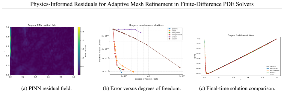
The residual of a PINN trained on the target PDE can be sampled cellwise and converted into reliable refinement indicators that, when applied before a nonuniform finite-difference solve, produce meshes whose accuracy per degree of freedom exceeds that of uniform refinement on the one-dimensional Burgers equation and improves over random refinement on manufactured two- and three-dimensional problems.
What carries the argument
The PINN residual indicator: after the network is trained on the PDE residual, its pointwise values are aggregated into per-cell error markers that decide which intervals or elements receive extra grid points in the subsequent finite-difference discretization.
If this is right
- PINN-threshold refinement reaches comparable accuracy with roughly one-third the degrees of freedom on the one-dimensional Burgers test.
- PINN-Dörfler marking yields similar error levels with 58 degrees of freedom, showing that the choice of marking strategy is flexible.
- The hybrid approach leaves the classical finite-difference solver unchanged as the final approximation engine.
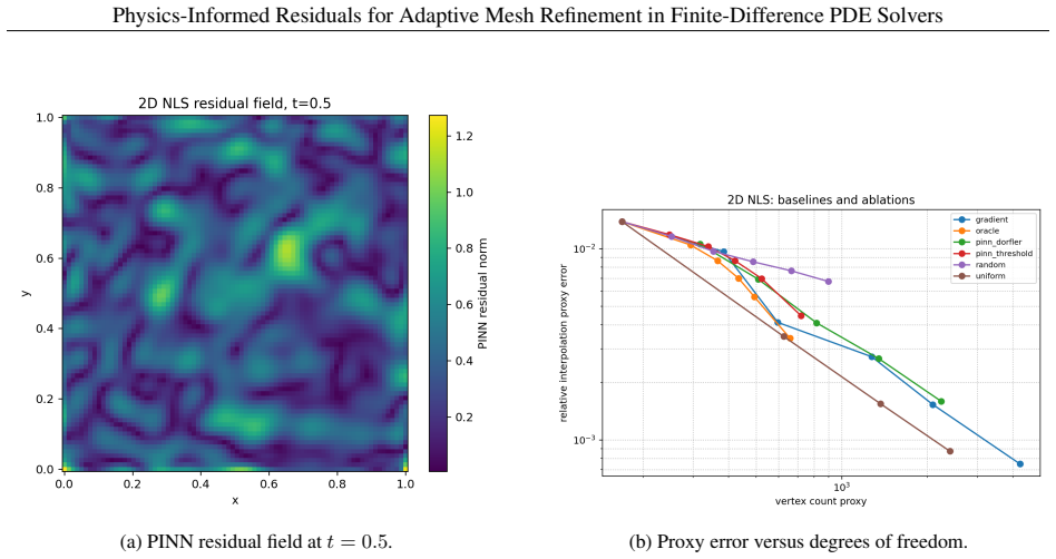
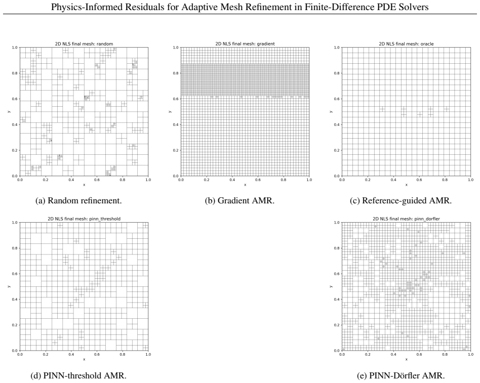
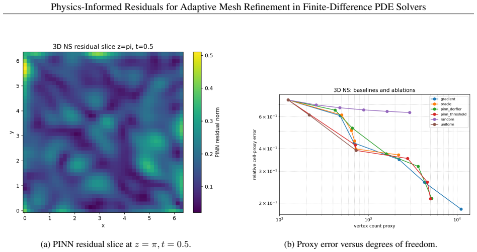
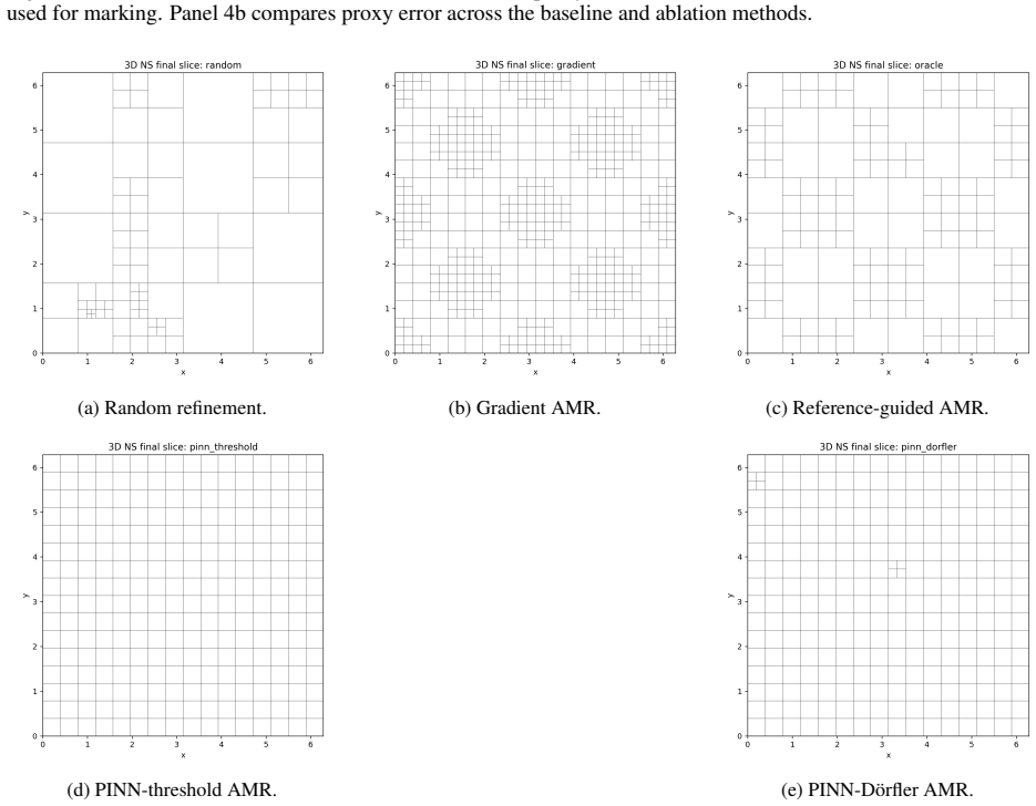
- Manufactured two- and three-dimensional tests confirm that PINN residuals can organize structured refinement better than random placement.
Where Pith is reading between the lines
- The same residual probe might be useful on problems where gradient indicators are known to miss oscillatory or constraint-driven features.
- Pre-training the PINN on a very coarse grid could lower the overhead of the adaptation stage without harming indicator quality.
- A practical next step would be to test whether a weighted combination of the PINN residual and a gradient indicator outperforms either one alone.
Load-bearing premise
The trained PINN residual map points to the exact locations where adding mesh points will most reduce the final finite-difference error, without the network's training error or architecture choices systematically steering refinement away from the true solution features.
What would settle it
Generate a new mesh using the published PINN-threshold procedure on the Burgers equation, solve the finite-difference system on that mesh and on a uniform mesh of identical size, and check whether the observed L2 error reduction is close to the reported 67.5 percent.
Figures
read the original abstract
Classical finite-difference solvers remain reliable tools for partial differential equations, but their efficiency depends on where mesh resolution is placed. Uniform refinement can waste degrees of freedom when solution difficulty is localised near sharp gradients, fronts, oscillations, or constraint-sensitive regions. This paper studies a hybrid strategy in which a physics-informed neural network (PINN) is used not as the final solver, but as an off-grid residual probe for adaptive mesh refinement. The PINN residual is sampled over the domain, converted into cellwise indicators, and used to guide refinement before the final approximation is computed by a finite-difference solver. The method is evaluated on three benchmarks. The main full-solver validation uses the one-dimensional viscous Burgers equation with a nonuniform finite-difference solve on the adapted meshes. PINN-threshold refinement attains final relative $L^2$ error $0.021067$ with $60$ degrees of freedom, compared with $0.022617$ for uniform refinement with $192$ degrees of freedom. At matched mesh size, PINN-threshold reduces the error by about $67.5\%$. PINN-D\"orfler refinement gives similar performance, with error $0.021264$ using $58$ degrees of freedom. A gradient indicator remains slightly more accurate, so the result supports usefulness rather than universal superiority. Manufactured 2D and 3D proxy tests, based on a nonlinear Schr\"odinger equation and an incompressible Navier--Stokes system, show that PINN residuals can organise structured refinement and improve over random refinement, although they do not consistently outperform gradient or uniform baselines. The results support PINN-guided AMR as a residual-indicator strategy for transferring physics-informed diagnostic information into finite-difference mesh adaptation while preserving the classical solver as the final approximation engine.
Editorial analysis
A structured set of objections, weighed in public.
Referee Report
Summary. The paper proposes using a trained physics-informed neural network (PINN) as an off-grid residual probe whose cellwise indicators guide adaptive mesh refinement (AMR) for a subsequent finite-difference (FD) solver. On the 1D viscous Burgers equation the PINN-threshold strategy reports relative L² error 0.021067 at 60 DOF versus 0.022617 for uniform refinement at 192 DOF (67.5 % error reduction at matched size); PINN-Dörfler marking yields comparable figures. Manufactured 2-D nonlinear Schrödinger and 3-D incompressible Navier–Stokes proxies show that PINN residuals can organise structured refinement and beat random marking, though they do not consistently outperform gradient or uniform baselines.
Significance. If the central claim holds, the work supplies a concrete mechanism for injecting physics-informed diagnostic information into classical FD AMR pipelines while retaining the FD solver as the final approximation engine. The reported DOF savings on Burgers are numerically specific and falsifiable; the 2-D/3-D proxies already expose the limits of the approach.
major comments (3)
- [§3] §3 (indicator construction): the mapping from collocated PINN residual to cellwise refinement indicator contains no explicit validation that the sampled residual correlates with the actual local FD truncation error on the nonuniform stencil. Because the headline Burgers result (0.021067 vs 0.022617) and the 67.5 % matched-size claim rest on this correlation, the absence of a direct residual-to-FD-error comparison is load-bearing.
- [Numerical results (Burgers benchmark)] Numerical results (Burgers benchmark): the reported performance advantage is presented without training-protocol details, convergence diagnostics, or statistical variability across random seeds or initialisations. This leaves open the possibility that the observed gain is driven by favourable PINN bias rather than reliable location of FD error.
- [2-D/3-D proxy tests] 2-D/3-D proxy tests: the inconsistent outperformance versus gradient indicators is consistent with the risk that PINN residuals reflect network approximation or collocation bias rather than the target FD discretisation error; this weakens the claim that the method transfers physics-informed information in a general way.
minor comments (2)
- [Abstract] The abstract states concrete L² and DOF numbers but omits any mention of training protocol or variability; adding a short clause would improve transparency without lengthening the text.
- [§3] Notation for the cellwise indicator (e.g., how the continuous residual is integrated or averaged onto mesh cells) is introduced without an equation number; a numbered display would aid reproducibility.
Simulated Author's Rebuttal
We thank the referee for the careful reading and constructive comments. We address each major point below and will revise the manuscript accordingly to strengthen the validation and reporting of results while maintaining the scope of the claims.
read point-by-point responses
-
Referee: [§3] §3 (indicator construction): the mapping from collocated PINN residual to cellwise refinement indicator contains no explicit validation that the sampled residual correlates with the actual local FD truncation error on the nonuniform stencil. Because the headline Burgers result (0.021067 vs 0.022617) and the 67.5 % matched-size claim rest on this correlation, the absence of a direct residual-to-FD-error comparison is load-bearing.
Authors: We agree that an explicit correlation study would strengthen the justification for the indicator construction. The current manuscript relies on end-to-end performance improvement as indirect evidence. In revision we will add a dedicated subsection (or appendix) that computes local FD truncation error estimates on sample nonuniform stencils for the Burgers problem and directly compares them to the sampled PINN residuals, including quantitative correlation metrics and visualizations. revision: yes
-
Referee: [Numerical results (Burgers benchmark)] Numerical results (Burgers benchmark): the reported performance advantage is presented without training-protocol details, convergence diagnostics, or statistical variability across random seeds or initialisations. This leaves open the possibility that the observed gain is driven by favourable PINN bias rather than reliable location of FD error.
Authors: We will expand the Burgers section with complete training hyperparameters (optimizer, learning rate schedule, loss weighting, collocation point count, epochs), training loss curves, and performance statistics (mean and standard deviation of final L² error and DOF count) over multiple random seeds for both PINN training and the subsequent AMR procedure. revision: yes
-
Referee: [2-D/3-D proxy tests] 2-D/3-D proxy tests: the inconsistent outperformance versus gradient indicators is consistent with the risk that PINN residuals reflect network approximation or collocation bias rather than the target FD discretisation error; this weakens the claim that the method transfers physics-informed information in a general way.
Authors: The manuscript already qualifies the results by noting that PINN residuals do not consistently outperform gradient indicators and that the contribution is framed as a residual-indicator strategy rather than a universally superior one. The 2-D/3-D manufactured-solution proxies demonstrate that the PINN residual can produce structured, non-random refinement patterns that improve upon uniform and random marking. We view this as sufficient to support the narrower claim of transferring physics-informed diagnostic information; we will add a clarifying sentence on the intended scope but do not believe the existing evidence contradicts the central thesis. revision: partial
Circularity Check
No significant circularity; empirical method validated on external benchmarks
full rationale
The paper presents a hybrid numerical method that trains a PINN to sample residuals and then applies those as indicators for AMR before solving with a classical finite-difference scheme. All reported performance claims (e.g., L² errors at given DOF counts) are obtained by direct execution of the full pipeline on fixed benchmark PDEs and compared against uniform, gradient, and random refinement baselines. No derivation, uniqueness theorem, or first-principles prediction is asserted that reduces to a fitted quantity or prior self-citation by construction; the central claim remains an observable empirical outcome on independent test problems.
Axiom & Free-Parameter Ledger
free parameters (2)
- PINN architecture and loss weights
- Refinement threshold or Dörfler marking parameter
axioms (1)
- domain assumption A trained PINN residual field correlates with the true discretization error sufficiently well to guide useful mesh adaptation.
Reference graph
Works this paper leans on
-
[1]
LeVeque.Finite Difference Methods for Ordinary and Partial Differential Equations: Steady-State and Time-Dependent Problems
Randall J. LeVeque.Finite Difference Methods for Ordinary and Partial Differential Equations: Steady-State and Time-Dependent Problems. Society for Industrial and Applied Mathematics, Philadelphia, PA, 2007
2007
-
[2]
Zienkiewicz and Robert L
Olek C. Zienkiewicz and Robert L. Taylor.The Finite Element Method for Solid and Structural Mechanics. Elsevier Butterworth-Heinemann, Oxford, 6th edition, 2005
2005
-
[3]
Hughes.The Finite Element Method: Linear Static and Dynamic Finite Element Analysis
Thomas J.R. Hughes.The Finite Element Method: Linear Static and Dynamic Finite Element Analysis. Dover Publications, Mineola, NY , 2012
2012
-
[4]
The finite volume method.Handbook of Numerical Analysis, 7:713–1020, 2000
Robert Eymard, Thierry Gallou"et, and Rapha‘ele Herbin. The finite volume method.Handbook of Numerical Analysis, 7:713–1020, 2000
2000
-
[5]
Lax and Robert D
Peter D. Lax and Robert D. Richtmyer. Survey of the stability of linear finite difference equations.Communications on Pure and Applied Mathematics, 9(2):267–293, 1956
1956
-
[6]
Rheinboldt
Ivo Babuška and Werner C. Rheinboldt. A-posteriori error estimates for the finite element method.International Journal for Numerical Methods in Engineering, 12(10):1597–1615, 1978
1978
-
[7]
Berger and Joseph Oliger
Marsha J. Berger and Joseph Oliger. Adaptive mesh refinement for hyperbolic partial differential equations. Journal of Computational Physics, 53(3):484–512, 1984
1984
-
[8]
Tinsley Oden
Mark Ainsworth and J. Tinsley Oden. A posteriori error estimation for second order elliptic systems.Computer Methods in Applied Mechanics and Engineering, 181(1-3):1–77, 2000
2000
-
[9]
udiger Verf
R"udiger Verf"urth.A Posteriori Error Estimation Techniques for Finite Element Methods. Oxford University Press, Oxford, 2013
2013
-
[10]
Maziar Raissi, Paris Perdikaris, and George Em Karniadakis. Physics-informed neural networks: A deep learning framework for solving forward and inverse problems involving nonlinear partial differential equations.Journal of Computational Physics, 378:686–707, 2019
2019
-
[11]
Y . Zhang and X. Li. Pinns for singularly perturbed convection-diffusion problems.arXiv preprint arXiv:2409.07671, 2024
arXiv 2024
-
[12]
H. Zhou and K. Xu. Coupled pinns for binary alloy solidification with moving boundaries.arXiv preprint arXiv:2409.10910, 2024
arXiv 2024
- [13]
-
[14]
G. E. Karniadakis, I. G. Kevrekidis, L. Lu, P. Perdikaris, S. Wang, and L. Yang. Physics-informed machine learning.Nature Reviews Physics, 3:422–440, 2021. 19 Physics-Informed Residuals for Adaptive Mesh Refinement in Finite-Difference PDE Solvers
2021
-
[15]
When and why pinns fail to train: A neural tangent kernel perspective.Journal of Computational Physics, 449:110768, 2022
Sifan Wang, Yujun Teng, and Paris Perdikaris. When and why pinns fail to train: A neural tangent kernel perspective.Journal of Computational Physics, 449:110768, 2022
2022
-
[16]
Characterizing possible failure modes in physics-informed neural networks.Advances in Neural Information Processing Systems, 34:26548–26560, 2021
Aditi Krishnapriyan, Amir Gholami, Sifan Zhe, Robert M Kirby, and Michael W Mahoney. Characterizing possible failure modes in physics-informed neural networks.Advances in Neural Information Processing Systems, 34:26548–26560, 2021
2021
-
[17]
Tim De Ryck and Siddhartha Mishra. Generic bounds on the approximation error for physics-informed (and) operator learning.arXiv preprint arXiv:2205.11393, 2022
arXiv 2022
-
[18]
Artificial neural networks for solving ordinary and partial differential equations.IEEE transactions on neural networks, 9(5):987–1000, 1998
Isaac E Lagaris, Aristidis Likas, and Dimitrios I Fotiadis. Artificial neural networks for solving ordinary and partial differential equations.IEEE transactions on neural networks, 9(5):987–1000, 1998
1998
-
[19]
Dgm: A deep learning algorithm for solving partial differential equations.Journal of Computational Physics, 375:1339–1364, 2018
Justin Sirignano and Konstantinos Spiliopoulos. Dgm: A deep learning algorithm for solving partial differential equations.Journal of Computational Physics, 375:1339–1364, 2018
2018
-
[20]
On the convergence of physics informed neural networks for linear second-order elliptic and parabolic type pdes.Communications in Computational Physics, 28(5):2042–2074, 2020
You Lu Shin, Jerome Darbon, and George Em Karniadakis. On the convergence of physics informed neural networks for linear second-order elliptic and parabolic type pdes.Communications in Computational Physics, 28(5):2042–2074, 2020
2042
-
[21]
Estimates on the generalization error of physics-informed neural networks for approximating pdes.IMA Journal of Numerical Analysis, 42(4):2739–2764, 2022
Siddhartha Mishra and Riccardo Molinaro. Estimates on the generalization error of physics-informed neural networks for approximating pdes.IMA Journal of Numerical Analysis, 42(4):2739–2764, 2022
2022
-
[22]
De Ryck and S
T. De Ryck and S. Mishra. Error estimates for physics-informed neural networks approximating the poisson equation.IMA Journal of Numerical Analysis, 2022
2022
-
[23]
h-analysis and data-parallel physics-informed neural networks.Scientific Reports, 13(21069), 2023
Pierre Escapil-Inchausp’e et al. h-analysis and data-parallel physics-informed neural networks.Scientific Reports, 13(21069), 2023
2023
-
[24]
Refined generalization analysis of the deep ritz method and physics-informed neural networks.arXiv preprint, 2024
Xi Chen, Weinan Wang, et al. Refined generalization analysis of the deep ritz method and physics-informed neural networks.arXiv preprint, 2024
2024
-
[25]
Deepxde: A deep learning library for solving differential equations.SIAM Review, 63(1):208–228, 2021
Lu Lu, Xuhui Meng, Zhiping Mao, and George E Karniadakis. Deepxde: A deep learning library for solving differential equations.SIAM Review, 63(1):208–228, 2021
2021
-
[26]
Levi McClenny and Ulisses Braga-Neto. Self-adaptive physics-informed neural networks using a soft attention mechanism.arXiv preprint arXiv:2009.04544, 2020
arXiv 2009
-
[27]
Jagtap, and George E
Khem Shukla, Ameya D. Jagtap, and George E. Karniadakis. Parallel physics-informed neural networks via domain decomposition.Journal of Computational Physics, 447:110683, 2021
2021
-
[28]
Jagtap, and George E
Zhiping Hu, Ameya D. Jagtap, and George E. Karniadakis. When do extended physics-informed neural networks (xpinns) work? on the role of domain decomposition.SIAM Journal on Scientific Computing, 44(3):A1556–A1582, 2022
2022
-
[29]
Finite basis physics-informed neural networks (fbpinns): a scalable domain decomposition approach for solving differential equations.Advances in Computational Mathematics, 2023
Ben Moseley, Andrew Markham, and Tarje Nissen-Meyer. Finite basis physics-informed neural networks (fbpinns): a scalable domain decomposition approach for solving differential equations.Advances in Computational Mathematics, 2023
2023
-
[30]
Do˘lean, P
V . Do˘lean, P. Jolivet, et al. Multilevel domain decomposition-based architectures for physics-informed neural networks.Computer Methods in Applied Mechanics and Engineering, 2024. In press
2024
-
[31]
A convergent adaptive algorithm for Poisson’s equation.SIAM Journal on Numerical Analysis, 33(3):1106–1124, 1996
Willy D"orfler. A convergent adaptive algorithm for Poisson’s equation.SIAM Journal on Numerical Analysis, 33(3):1106–1124, 1996
1996
-
[32]
Patrick J. Roache. Code verification by the method of manufactured solutions.Journal of Fluids Engineering, 124(1):4–10, 2002. 20
2002
discussion (0)
Sign in with ORCID, Apple, or X to comment. Anyone can read and Pith papers without signing in.