REVIEW 4 major objections 4 minor 9 references
The Study on Modified Theories of General Relativity: A Differential Geometric Approach
T0 review · 4 major / 4 minor · reviewed 2026-08-06 · deepseek-v4-flash
Pith's one-line read The thesis claims that modified gravity built from non-metricity, torsion, and matter-coupled curvature can reproduce ΛCDM expansion, support traversable wormholes, and pass BBN plus late-time tests.
desk verdict A PhD thesis compiled from published papers, with a load-bearing flaw in the f(R,L_m) chapters: the action is complex-valued for the fitted parameters, and the ΛCDM embedding is by construction rather than an independent test. read the letter →
The pith
A machine-rendered reading of the paper's core claim, the machinery that carries it, and where it could break.
The reading
What carries the argument
The load-bearing construction is the replacement of the linear Ricci scalar in the Einstein-Hilbert action by arbitrary functions of geometric invariants: $f(Q)$ for non-metricity, $f(T)$ for torsion, $f(R,L_m)$ and $f(Q,L_m)$ for curvature or non-metricity coupled to the matter Lagrangian, and $f(Q,T)$ for non-metricity coupled to the trace of the stress-energy tensor. Varying these actions with respect to metric and connection yields modified Friedmann and wormhole equations. In the wormhole chapters the decisive mechanism is the conformal Killing vector condition, $\mathcal{L}_\eta g_{ab}=\psi(r)g_{ab}$, which turns the non-linear field equations into ordinary differential equations whose solution gives the wormhole shape function $S_f(r)$; in the $f(R,L_m)$ wormhole chapter, non-commutative Gaussian and Lorentzian smearing of the energy density plays the same role. In the reconstruction chapters the decisive object is the first-order differential equation obtained by inserting the ΛCDM form of the non-metricity scalar into the modified Friedmann equation, whose closed-form solution yields the geometric function $f_1(Q)$ for a prescribed coupling $f_2(Q)$.
What would settle it
Compute $(-\rho)^\alpha$ at the best-fit value $\alpha=4.76$ and a positive cosmological density; unless the paper specifies which branch of the complex power is meant, the field equations (4.18)-(4.20) do not follow from a real action, and the Chapter 4 and Chapter 6 results are undefined before comparison with data.
Extended reading notes
Core claim
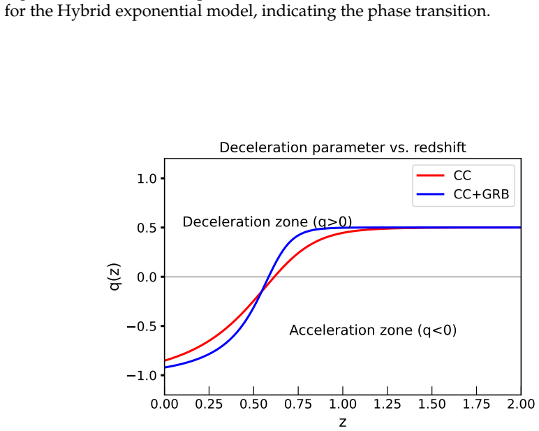
The central claim is that the geometric trinity of general relativity, built on curvature, torsion, and non-metricity, admits modified extensions whose actions produce the observed cosmic history and support wormhole geometries. In the $f(Q)$ chapter, the thesis derives the deceleration parameter $q(z)=-1+a(1+z)^3/(z^3+5z^2+b)$ with best-fit values $a=1.513$, $b=5.04$, $H_0=74.43\, \mathrm{km\,s^{-1}Mpc^{-1}}$, and reconstructs power-law and logarithmic $f(Q)$ forms whose effective evolution tracks ΛCDM. In the non-minimally coupled $f(Q,L_m)$ chapter, it solves the reconstruction equation analytically for power-law and logarithmic couplings, obtaining the geometric function $f_1(Q)$ that makes the background expansion exactly ΛCDM, and validates the coefficients cosmographically with Pantheon+ data. In the $f(R,L_m)$ Bianchi-I chapter, the equation of state is fitted to Hubble and Pantheon samples and found to be phantom-like, with a small anisotropy parameter. The wormhole chapters show that in $f(Q,T)=\alpha Q+\beta T$ with conformal symmetry, three equations of state yield shape functions satisfying the throat and flare-out conditions, with the anisotropic case satisfying both null energy conditions, while in $f(R,L_m)$ Gaussian and Lorentzian non-commutative profiles yield wormhole shape functions and energy-condition analyses. The final chapter constrains two hybrid $f(T)$ models so that their BBN predictions and late-time cosmic-chronometer plus gamma-ray-burst data leave overlapping parameter ranges, with intermediate epochs checked by cosmography.
Load-bearing premise
The load-bearing premise is that $L_m=-\rho$ may be used in $f(R,L_m)=R/2+L_m^\alpha$ with non-integer fitted exponents $\alpha$, so that $(-\rho)^\alpha$ is interpreted as a real number even though ordinary exponent rules give a complex value for positive $\rho$.
Editorial extensions
If this is right
- If the reconstructed $f(Q)$ forms are correct, the same expansion data that support ΛCDM are reproduced by non-metricity-based gravity without a cosmological constant term in the action.
- If the $f(Q,L_m)$ embedding holds, the ΛCDM background can be realized exactly by a non-minimal geometry-matter coupling, so late-time acceleration need not require a vacuum-energy cosmological constant.
- If the conformally symmetric $f(Q,T)$ wormholes are genuine solutions, traversable wormholes can exist with ordinary non-exotic matter in the anisotropic-pressure case, making the exotic-matter obstacle model-dependent.
- If the hybrid $f(T)$ models pass BBN and late-time constraints, teleparallel gravity offers an early-to-late cosmological viability with model parameters confined by overlapping early- and late-time bounds.
- If the Bianchi-I $f(R,L_m)$ fit is reliable, a small but measurable anisotropy is compatible with the same Hubble and Pantheon samples used to support an accelerating Universe.
Reading between the lines
- A natural next test the thesis does not perform is perturbation theory: background equivalence to ΛCDM in $f(Q,L_m)$ does not guarantee the same growth of structure, so cosmic-shear and redshift-space-distortion data could discriminate the models.
- The $f(Q)$ reconstruction in Chapter 2 is anchored to $H_0\approx 74.4\, \mathrm{km\,s^{-1}Mpc^{-1}}$; if the Hubble tension resolves toward the lower Planck value, the fitted $\alpha,\beta$ values change and the models' apparent closeness to ΛCDM may weaken.
- For the $f(R,L_m)$ wormholes, the non-commutative profiles are assumed in the form of Gaussian and Lorentzian smearing; a decisive extension would derive such profiles from the theory's own minimal-length structure rather than impose them.
- The BBN constraint pipeline could be applied to the non-metricity theories as well: the same $\Delta T_F/T_F$ bound plus cosmography would give an early-time test for $f(Q)$ and $f(Q,T)$, not only for $f(T)$.
Signed reviews
Editorial analysis
A structured set of objections, weighed in public.
Referee Report
Summary. The manuscript is a PhD thesis compilation, arXiv:2507.04031, presenting seven chapters on modified theories of gravity. It introduces a two-parameter deceleration parameter and uses it to reconstruct f(Q) models (Chapter 2), embeds the ΛCDM expansion history into non-minimally coupled f(Q,L_m) gravity by solving for the functions f1 and f2 (Chapter 3), studies LRS Bianchi-I cosmological models in f(R,L_m)=R/2+L_m^alpha (Chapter 4), constructs wormhole solutions in f(Q,T) gravity with conformal symmetries (Chapter 5), repeats the f(R,L_m) wormhole analysis with non-commutative geometry (Chapter 6), and constrains hybrid f(T) models using Big Bang Nucleosynthesis and late-time data (Chapter 7). The abstract and preface claim that these modified gravity theories are viable frameworks for cosmic acceleration, traversable wormholes (in one case without exotic matter), and BBN-compatible late-time cosmology.
Significance. If the collection is correct, it would provide a menu of modified gravity models that all reproduce the background expansion history and yield explicit wormhole solutions, with the f(T) chapter providing cross-checks between early- and late-time constraints. The strengths of the manuscript include the use of current observational datasets (Pantheon+, CC, BAO), MCMC parameter estimation, explicit analytic reconstruction formulas in Chapters 2 and 3, and a reasonably complete energy-condition analysis in the wormhole chapters. The thesis is also grounded in a series of already-published papers, which lends some confidence that the individual calculations were externally reviewed. However, the load-bearing issues identified below—especially the complex-valued f(R,L_m) action—mean that the central viability claims are not currently supported as stated.
major comments (4)
- [Chapter 4, Eq. (4.13) and Table 4.1; Chapter 6, Eqs. (6.1)-(6.4)] The action f(R,L_m)=R/2+L_m^alpha with L_m=-rho and positive rho is not real-valued for the fitted non-integer alpha values (4.76, 5.57, 6.4). In Eq. (4.18)-(4.20) the term (-rho)^alpha appears explicitly; for alpha not an integer this is complex, so the field equations do not follow from a real stationary action. No branch convention or real-part prescription is stated anywhere in Chapters 4 or 6. Since the MCMC constraints, the reconstructed H(z), and the wormhole energy-condition results all depend on Eqs. (4.18)-(4.20), the f(R,L_m)-based conclusions are invalid as stated. The authors should either restrict alpha to integers (or odd integers, e.g. alpha=5), adopt and justify a specific branch of the complex power, or replace the model with a manifestly real Lagrangian, and then redo the fits and wormhole analysis.
- [Chapter 3, Eq. (3.13); Chapter 2, Eqs. (2.22)-(2.23)] The 'embedding' of ΛCDM into f(Q,L_m) is a reconstruction by construction: Eq. (3.13) is the ΛCDM Friedmann equation rewritten in terms of Q, and f1 and f2 are then solved so that the resulting model reproduces the assumed H(z). Consequently the analytic solutions in Sections 3.5.1-3.5.3 do not independently test against ΛCDM; agreement is guaranteed by the construction. Similarly, in Chapter 2 the parameters (alpha, beta) of the f(Q) models are computed from the fitted q0, H0, and an externally fixed Omega_m0 via Eqs. (2.22)-(2.23), so the reconstructed f(Q) curves are consistency checks rather than falsifiable predictions. The chapters should state this limitation explicitly and temper the viability language accordingly.
- [Chapter 5, Sections 5.5.1-5.5.3 and Eqs. (5.10)-(5.24)] The wormhole solutions are not asymptotically flat, as the authors themselves note after Eq. (5.24): S_f/r tends to a non-zero constant (e.g. (8 beta + 6)/(10 beta + 9) in Case 1), so the spatial metric approaches a conical or constant-deficit geometry rather than Minkowski space at infinity. For standard Morris-Thorne traversable wormholes, asymptotic flatness is one of the defining boundary conditions. The claims that these are physically viable traversable wormhole solutions therefore require either a matching to an exterior flat region or a clear statement that these are wormhole-like configurations in a non-asymptotically-flat background, which changes their physical interpretation.
- [Chapter 4, Table 4.1 and Eq. (4.25)] The fitted anisotropy parameter Delta is of order 1.6, and the directional Hubble ratio n is of order 27-31. This means the directional expansion rates differ by a factor of about 27, which is difficult to reconcile with the chapter's stated motivation that the Universe has only very small large-scale anisotropy. The text claims the model predicts an anisotropy 'in agreement with the dataset used' (Section 4.6), but no comparison is made with observational bounds on cosmological anisotropy (e.g. CMB quadrupole or shear constraints). The conclusion that the model is consistent with observed isotropy is therefore unsupported; the authors should either compare Delta with actual bounds or refrain from that claim.
minor comments (4)
- [Front matter] The manuscript contains university declaration pages, a plagiarism report, and submission metadata. These are inappropriate for a journal article and should be removed or moved to a supplementary file.
- [Throughout] The text contains typographical errors and inconsistent notation, e.g. 'Covarient' (Section 1.2), 'Christeffol' (Section 1.5.2.2), and the use of both 'article' and 'chapter' for self-reference. A thorough proofread is needed.
- [Chapter 5, Eq. (5.1)] The action in Eq. (5.1) has a formatting error: 'SM = R Lm sqrt(-g) d4x f(Q,T)' is not a well-formed expression. The intended definition of the matter action and the f(Q,T) model should be written explicitly.
- [Chapter 3, Sections 3.5-3.6] The hypergeometric and regularized hypergeometric function expressions (e.g. Eqs. (3.18), (3.23), (3.28)) are written without specifying their domains of convergence or the allowed parameter ranges; since these formulas are central to the reconstruction, a brief statement on parameter validity would help the reader.
Circularity Check
Chapters 2 and 3 reduce by construction: f(Q) parameters are solved from the fitted q0/H0/Omega_m0, and f1/f2 are solved from the LambdaCDM Hubble rate; the rest of the thesis is mostly self-constrained model fitting rather than circular.
-
self definitional
[Chapter 3, Sections 3.4-3.5, Eq. (3.13) and Eq. (3.18)/(3.19)]
"To derive fi’s that replicate the ΛCDM expansion, it is necessary to incorporate all of the relevant parameters expressed as functions of the non-metricity scalar into the Friedmann equation (3.4). Now, substituting all the parameters in terms of Q into (3.4), we obtain a first-order inhomogeneous differential equation, expressed as follows Q/2 = ... (3.13)."
Equation (3.13) is the Friedmann equation (3.4) evaluated with the ΛCDM Hubble function inserted via (3.8)-(3.12). The functions f1 and f2 are then obtained as solutions of this very differential equation, so the later statement that the model "would accurately replicate the expansion history of the ΛCDM model" is the input ansatz returned after solving an equation that already contains ΛCDM. No independent ΛCDM-like expansion is predicted; it is enforced by construction.
-
fitted input called prediction
[Chapter 2, Section 2.7, Eqs. (2.19)-(2.26), Table 2.3, Figs. 2.8-2.9]
"By substituting the values q0 = −0.7, H0 = 74.43 obtained in this study along with Ωm0 = 0.315 [44], into Equations (2.22) and (2.23), we find the corresponding parameter values for the power-law f (Q) gravity model as α = 0.255708 and β = −0.839416."
The parameters α and β are not constrained by an independent prediction of the f(Q) model; they are algebraically solved from the two present-day Friedmann equations (2.22)-(2.23) after inserting the MCMC-fitted q0 and H0 together with an adopted Ωm0. The reconstructed f(Q) curves in Figs. 2.8-2.9 are therefore a repackaging of those fitted inputs, and the comparison with ΛCDM is a consistency check rather than a test. The logarithmic model is treated identically via (2.25)-(2.26).
full rationale
The clearest circularity is in Chapter 3. Equation (3.13) is the f(Q,Lm) Friedmann equation with the ΛCDM H(Q) substituted; the paper then solves that differential equation for f1 or f2. The claim that the resulting theory 'replicates' ΛCDM is therefore true by construction, not by empirical test. Chapter 2 has a milder but real version: α and β for the two f(Q) ansatze are obtained by solving the present-day Friedmann equations with the MCMC-fitted q0, H0, and an adopted Ωm0, so the reconstructed f(Q) curves are functions of those inputs; comparing them with ΛCDM is a self-consistency check. The other chapters — Bianchi-I f(R,Lm), wormholes in f(Q,T) and f(R,Lm), BBN in f(T) — fit their parameters to the data they then display, which is normal likelihood-based model validation rather than circularity in the sense of this review. No load-bearing self-citation chain was found. A separate correctness issue, not a circularity, is that Chapter 4's model f = R/2 + L_m^α with L_m = -ρ and fitted non-integer α makes (-ρ)^α complex, so Eqs. (4.18)-(4.20) require an unstated branch choice; this affects viability but does not by itself make the derivation circular.
Assumptions & free parameters
free parameters (15)
- a in q(z) parametrization =
1.513+0.073/-0.073
- b in q(z) parametrization =
5.04+0.37/-0.44
- H0 in Chapter 2 =
74.43+0.18/-0.18 km/s/Mpc
- alpha in power-law f(Q) model =
0.255708
- beta in power-law f(Q) model =
-0.839416
- alpha in logarithmic f(Q) model =
1.155
- beta in logarithmic f(Q) model =
-0.42
- f(Q,Lm) power-law case parameters =
xi=-1.28, nu=0.801, F1=2.23849e4, F2=0.073, F3=0.85, F4=0.01, H0=78.3, Omega_m0=0.316
- f(Q,Lm) logarithmic case parameters =
xi=-1.19, F1=-4.0411e3, F2=-0.073, F3=0.85, F4=0.012, H0=79.35, Omega_m0=0.299
- w (EoS parameter) in f(R,Lm) =
-1.245 (H(z)), -1.175 (Pantheon), -1.281 (H(z)+Pantheon)
- alpha in f(R,Lm) model =
5.57 (H(z)), 6.4 (Pantheon), 4.76 (H(z)+Pantheon)
- n in Bianchi-I anisotropy relation =
26.73 (H(z)), 31.09 (Pantheon), 28.65 (H(z)+Pantheon)
- Chapter 5 wormhole parameters =
alpha=1.5, beta=0.9, C2=2, r0=1, w=0.4 (Case 3); alpha=1.4, C2=1.26, r0=0.35, A=2.25 (Case 2)
- Chapter 6 non-commutative wormhole parameters =
M=1.2, theta=4, r0=1, alpha varied
- Chapter 7 f(T) hybrid model parameters =
n (hybrid exponential) and a (hybrid tanh), ranges in Table 7.2
assumptions (10)
- standard math Standard differential geometry definitions and tensor calculus are assumed.
- standard math Einstein field equations and the LambdaCDM expansion history are taken as baseline.
- domain assumption Cosmological chapters use a flat FLRW or LRS Bianchi-I background.
- domain assumption Matter is modeled as a perfect fluid with barotropic equation of state p=w rho.
- domain assumption The matter Lagrangian is chosen as Lm=p in f(Q,Lm) and Lm=-rho in f(R,Lm).
- ad hoc to paper The deceleration parameter has the assumed form q(z)=-1+a(1+z)^3/(z^3+5z^2+b).
- ad hoc to paper Specific Lagrangian forms are assumed: power/log f(Q), power/log f2 in f(Q,Lm), f(R,Lm)=R/2+L_m^alpha, f(Q,T)=alpha Q+beta T, and hybrid f(T) models.
- ad hoc to paper Wormhole chapters impose conformal Killing vectors and non-commutative Gaussian or Lorentzian profiles.
- ad hoc to paper The expression (-rho)^alpha is treated as real for positive rho and non-integer alpha.
- domain assumption Standard Big Bang nucleosynthesis abundance predictions are valid and f(T) corrections are small perturbations.
Cite this review
Pith. "Pith review of The Study on Modified Theories of General Relativity: A Differential Geometric Approach." pith.science (2026). https://pith.science/paper/QVQUOQHX
@misc{pith2026250704031,
  author       = {Pith},
  title        = {Pith review of: The Study on Modified Theories of General Relativity: A Differential Geometric Approach},
  year         = {2026},
  howpublished = {\url{https://pith.science/paper/QVQUOQHX}},
  note         = {Machine review of arXiv:2507.04031}
}
read the original abstract
The introduction of General Relativity (GR) in 1915 revolutionized our understanding of gravity, but over time, its limitations in explaining phenomena like dark energy, dark matter, and quantum gravity have motivated alternative theories. Early modifications, such as Weyl's 1919 proposal, focused on adding higher-order terms to the Einstein-Hilbert action. GR's non-renormalizability further strengthened the case for extending it. A central theme of modern gravity research is modifying the geometric structure, often by changing the gravitational Lagrangian. This leads to theories such as teleparallel and symmetric teleparallel gravity, utilizing torsion or non-Levi-Civita connections, with differential geometry providing the essential framework. This thesis explores several modified gravity models. Chapter 1 introduces necessary mathematical tools. Chapter 2 develops a novel parametrization of the deceleration parameter, constrained using MCMC and observational data, and applies it to f(Q) gravity. Chapter 3 embeds the LambdaCDM model into f(Q, L\_m) gravity with non-minimal coupling, producing analytic solutions and matching observations through cosmographic analysis. Chapter 4 considers Bianchi-I spacetime in f(R, L\_m) gravity with observational constraints to measure anisotropy. Chapter 5 presents wormhole solutions in f(Q, T) gravity with conformal symmetries. Chapter 6 explores wormholes in f(R, L\_m) with non-commutative geometry, analyzing shape functions, energy conditions, and stability. Chapter 7 studies Big Bang Nucleosynthesis in f(T) gravity, constraining hybrid models using early- and late-time data, and validating intermediate epochs via cosmography.
Figures


Figures from the paper (72 more)




Reference graph
Works this paper leans on
-
[1]
Introduction A prominent challenge in contemporary cosmology is the need for a profound explanation of the origin and existence of the dark components of the Universe, which are accountable for the observed acceleration of the Universe supported by recent observations [39,40]. To address this, introducing a cosmological constant Λinto Einstein’s equations...
-
[8]
Introduction Overthepastfewdecades,manyscientificexplorationshave beentakingplacetodecipherthemysticbehavioroftheuniverse. Rightfromtheearlytimeinflationtothelatetimeacceleration, fromtheblackholestothewormholes,fromthedarkenergyto thegravitationalwaves,theirentirecoursehasbeenprobingthe verynatureoftheuniverse.Justtolookintothecosmological principle,theu...
arXiv 2023
-
[9]
Introduction Wormholes are unique geometric structures in the realm of theoretical physics, representing classical or quantum solutions to gravitational field equations. They offer the possibility of connecting two distant regions through a bridge-like pathway. In classical terms, they can be similar to instantons, representing tunneling events between as...
-
[269]
Quasar-Lyman α Forest Cross-Correlation from BOSS DR11 : Baryon Acoustic Oscillations,
A. Font-Ribera et al. , “Quasar-Lyman α Forest Cross-Correlation from BOSS DR11 : Baryon Acoustic Oscillations,” JCAP, vol. 05, p. 027, 2014. DOI: 10 . 1088/1475-7516/2014/05/027. arXiv: 1311.1767 [astro-ph.CO]
arXiv 2014
-
[270]
Measurement of baryon acoustic oscillation correlations at z = 2.3 with SDSS DR12 Lyα-Forests,
J. E. Bautista et al. , “Measurement of baryon acoustic oscillation correlations at z = 2.3 with SDSS DR12 Lyα-Forests,” Astron. Astrophys., vol. 603, A12, 2017. DOI: 10.1051/0004-6361/201730533. arXiv: 1702.00176 [astro-ph.CO]
arXiv 2017
-
[271]
Y. Wang et al., “The clustering of galaxies in the completed SDSS-III Baryon Os- cillation Spectroscopic Survey: tomographic BAO analysis of DR12 combined sample in configuration space,” Mon. Not. Roy. Astron. Soc. , vol. 469, no. 3, pp. 3762–3774, 2017. DOI: 10 . 1093 / mnras / stx1090. arXiv: 1607 . 03154 [astro-ph.CO]
work page 2017
-
[272]
The clustering of the SDSS DR7 main Galaxy sample – I. A 4 per cent distance measure at z = 0.15,
A. J. Ross, L. Samushia, C. Howlett, W. J. Percival, A. Burden, and M. Manera, “The clustering of the SDSS DR7 main Galaxy sample – I. A 4 per cent distance measure at z = 0.15,” Mon. Not. Roy. Astron. Soc. , vol. 449, no. 1, pp. 835–847,
-
[273]
Intrinsic spectra and energetics of BeppoSAX gamma-ray bursts with known redshifts,
L. Amati et al., “Intrinsic spectra and energetics of BeppoSAX gamma-ray bursts with known redshifts,” Astron. Astrophys., vol. 390, p. 81, 2002. DOI: 10.1051/ 0004-6361:20020722. arXiv: astro-ph/0205230. 196 APPENDIX Cosmological Developments and Surveys Throughout the 20th and early 21st centuries, remarkable milestones have shaped our understanding of ...
arXiv 2024
Show all 9 references
- [2015]
Reviewed August 6, 2026 · model on record in the stance chip above.
Discussion (0). Continue with ORCID to comment.