REVIEW 4 major objections 4 minor 46 references
Dynamical Optimal Transport with $\mathfrak{so}(d)$-Invariance: From Theory to Computation
T0 review · 4 major / 4 minor · reviewed 2026-08-01 · deepseek-v4-flash
Pith's one-line read A transport metric that makes rigid motions free equals the static Procrustes–Wasserstein distance.
desk verdict Core math is sound and the dynamic-static equivalence is a genuine contribution; the numerical half is not yet connected to the theory, but the paper deserves a serious referee. read the letter →
The pith
A machine-rendered reading of the paper's core claim, the machinery that carries it, and where it could break.
The reading
What carries the argument
The key object is the MBB seminorm on the Wasserstein tangent space. For each measure μ it projects a velocity field onto the orthogonal complement of the finite-dimensional space of rigid fields x ↦ Ex + C, with E skew-symmetric. The dynamical action is the integral of this projected norm squared. The dynamic–static equivalence is carried by the rigid flow g_t(x)=Q_t x + b_t generated by (E,C); pulling back the measure curve by g_t converts the MBB action into classical Benamou–Brenier action between aligned endpoints, which then realizes the static Procrustes–Wasserstein distance.
What would settle it
Take two identical radially symmetric densities on a fixed grid and run the alternating scheme: the action is zero for any skew-symmetric field E, so the inner residual can vanish while E varies. If the algorithm produces unbounded or initialization-dependent E sequences, or if the stability constant in Section 8 blows up as shown for perturbed radial densities, the local branch assumption behind the convergence theorem is violated.
Extended reading notes
Core claim
The central claim is Theorem 1: for any two probability measures with finite second moments, the modified Benamou–Brenier value—built by assigning zero energy to the rigid component of the velocity field—equals the orientation-preserving Procrustes–Wasserstein distance, i.e. the minimum of the squared Wasserstein distance after applying a special Euclidean isometry to one measure. The proof uses a rigid flow that 'undoes' the rotation and translation, pulling back the dynamics to a classical Benamou–Brenier problem and then optimizing over the final isometry. Theorem 4 gives the Gaussian closed form: the distance equals the Euclidean norm of the difference between the square roots of the ord
Load-bearing premise
The computational convergence theorem rests on the unverified premise that the iterates remain in a local regularity neighborhood and that at the reference solution the effective non-rigid velocity satisfies a smallness condition (C_h ||m*/ρ* − Π0 g_{E*}||_∞ < c_h); if either fails, the scheme may not converge to a stationary point.
Editorial extensions
If this is right
- The equivalence reduces computation of the MBB distance to a two-step problem: first align optimally, then compute classical Wasserstein distance.
- For Gaussians, Procrustes–Wasserstein distance can be computed in closed form by sorting and square-rooting eigenvalues, enabling fast alignment and comparison of normal distributions.
- The quotient space of centered measures modulo rotations is a complete, path-connected, geodesic metric space; geodesics in the quotient can be realized by projecting Wasserstein geodesics after optimal alignment.
- Under the stated local regularity and smallness conditions, the alternating primal–dual algorithm yields accumulation points that satisfy the discrete optimality conditions.
- The full Procrustes–Wasserstein distance is obtained by taking the minimum of two orientation-preserving MBB values, one with a reflected target, so the computational scheme extends to orientation-reversing comparisons.
Reading between the lines
- The dynamic–static equivalence suggests that the MBB action is the natural kinetic energy on the quotient of Wasserstein space by Euclidean isometries, so gradient flows in this quotient could serve as principled shape interpolations.
- Because the recovered rotation generator suffers from a gauge-type nonuniqueness near symmetric densities, any practical solver that produces a rotation path will need an explicit gauge or regularization if that path is to be meaningful.
- A testable extension beyond Gaussians: for elliptically symmetric or log-concave families, the eigenvalue-square-root distance might emerge as an approximation; numerical experiments could check whether alignment reduces to eigendecomposition for those measures.
Signed reviews
Editorial analysis
A structured set of objections, weighed in public.
Referee Report
Summary. The paper introduces a Modified Benamou–Brenier (MBB) formulation of optimal transport in which only the non-rigid part of the velocity field is penalized, so that the dynamics is invariant under the special Euclidean group SE(d). The central theoretical result, Theorem 1, proves that the MBB value equals the static orientation-preserving Procrustes–Wasserstein distance d_S, with an analogous statement for the full orthogonal group; Theorem 2 gives existence of static and dynamic minimizers. For Gaussian measures, Theorem 4 derives the closed form d̄² = ||√a₀ − √a₁||², where a₀, a₁ are the ordered eigenvalues of the covariance matrices. The second half of the paper develops an abstract conditional local convergence framework for parameter-dependent saddle-point problems (Section 5) and applies it to a fixed-grid discretization of the MBB problem, yielding the conditional subsequential convergence result Theorem 7. Numerical experiments on 2D densities illustrate the scheme. The paper is explicit about the conditional nature of the computational result in Remarks 11–12 and in Section 8.
Significance. If the main theoretical results stand, they are a clean and useful contribution: the dynamic–static equivalence in Theorem 1 is proved by an elegant rigid-flow change of variables, and the Gaussian closed form in Theorem 4 is a compact, usable formula. The paper also re-derives the Gaussian result independently rather than importing it. The abstract saddle-point analysis in Section 5 is a reasonable, carefully stated local convergence framework. However, the computational half is currently not connected to the theory: the numerical experiments do not verify the hypotheses of Theorem 7, and a central benchmark (pure rotation) recovers only about 33° instead of the nominal 45°, which contradicts the qualitative claim that the scheme 'correctly captures a purely rotational motion.' The paper's honest caveats are a strength, but they imply that the reported computations are numerical illustrations rather than a validated instantiation of the convergence theorem.
major comments (4)
- [§7.5, Theorem 7, Eq. (56)–(57)] The experiments do not instantiate Theorem 7. The theorem requires the residual-based acceptance rule (56) with a summable tolerance sequence, fixed step sizes satisfying Corollary 3 and Proposition 5, and iterates remaining in the local neighborhoods (57). Section 7.5 instead uses a fixed inner iteration cap of five PDHG steps, an outer horizon of 500, adaptive residual-balancing step sizes, and a stopping/diagnostic criterion based on outer iterate differences. Thus the convergence guarantee of Theorem 7 does not apply to the reported numerical results, and the paper's 'From Theory to Computation' claim is not supported on the computational side.
- [§7.1, Lemmas 11 and 18, Proposition 7] The discretization used in the experiments violates an explicit hypothesis of the theory. Section 7.1 states n_t = 64 grid points in time with h_t = 1/(n_t−1), which gives K = 63 time intervals, an odd number. Lemma 11, Lemma 18, and Proposition 7 all explicitly assume that K is even. Consequently, the discrete compatibility, coercivity, and Assumption 2 results in Section 6 do not apply to the grid used in the numerical section, independently of the inner/outer loop choices.
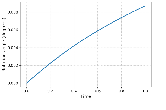
- [§7.2, Figure 5 and Discussion] The pure-rotation benchmark recovers an angle of approximately 33° instead of the nominal 45°. This is a large error for a configuration that should be absorbed entirely by the orthogonal component at zero transport cost. The text attributes the discrepancy to numerical effects, but does not provide any quantitative error analysis or explain why the optimizer stops at 33°. This undermines the claim in the Discussion that the MBB formulation 'correctly captures a purely rotational motion' and also calls into question the meaning of the reported kinetic-energy comparison, since a suboptimal E would require a compensating V with non-negligible energy.
- [§8, Examples 1–2] The paper's own stability analysis shows that the linearized E-operator has a kernel at radial densities (Example 1) and that arbitrarily small non-symmetric perturbations produce a stability constant growing like 1/ε (Example 2). Hence the local neighborhoods U_{E*} × U_{z*} required by condition (57) may be arbitrarily small near symmetric inputs, and the smallness condition (48) in Proposition 7 is not verified anywhere. The convergence theorem is therefore not only conditional but also potentially inapplicable precisely in regimes close to the type of data used in the experiments. The section honestly explains why local analysis is needed, but it also underscores that the computational claims are not validated.
minor comments (4)
- [Theorem 4, proof] The proof would benefit from stating explicitly that the eigenvector matrices P₀, P₁ are chosen with matching orientation (det P₀ = det P₁) so that the optimal transformation P₁P₀ᵀ lies in SO(d). As written, the statement 'optimal orthogonal transformation' is ambiguous when arbitrary eigendecompositions are used.
- [§7, Figures 3, 8, 13] The quantity plotted as 'fixed-point residual' is not defined in the experimental section. The paper should specify the exact residual norm being computed in the figures, since this is not the residual Res in (29) used in the theory.
- [Remark 6] Remark 6 says 'As shown in Lemma 9, the variables split into three blocks'; Lemma 9 concerns convex-concave structure, not the block splitting. The reference should be to the algorithmic presentation in Section 4.2.
- [§7.5] The text states that the adaptive step-size strategy is used 'only in the implementation' and that the theory requires fixed step sizes. This is an important caveat, but it is placed late and should be emphasized more prominently in the numerical section to avoid any impression that the experiments verify the convergence theorem.
Circularity Check
No significant circularity: the dynamic–static equivalence and the Gaussian closed form are derived in-paper from definitions and standard OT theory; the only signal is a minor, non-load-bearing self-citation of [43].
full rationale
The paper's main derivation chain is self-contained. Theorem 1 proves that the MBB dynamic value equals the static orientation-preserving Procrustes–Wasserstein distance by two constructive inequalities: (I) pulling an admissible (mu,V,E,C) back through the rigid flow generated by (E,C) (Lemmas 5–6) and invoking the classical Benamou–Brenier characterization [7] to get d_S^2 <= J; (II) given a BB geodesic to (Q,b)#mu1, lifting it forward through a rigid path in SE(d) with E_t = dQ_t Q_t^T, C_t = db_t - E_t b_t to produce an admissible quadruple with equal action. No parameter is fitted and no quantity is defined in terms of the conclusion; the equality is a genuine theorem, and its two directions use invertible explicit maps rather than a tautology. Theorem 4 (Gaussian closed form) is also proved in the paper: after centering and eigendecomposition, F(theta) = sum sigma_i(A1^{1/2} Theta A0^{1/2}) is bounded above by <sqrt a0, sqrt a1> via the external singular-value inequality [28, Thm. 3.3.14], and the bound is attained at Theta = I, giving the stated eigenvalue formula. The statements 'A preliminary version of this result appeared in [43]' and 'as announced in [43]' are the only self-citations; because the proof is fully reproduced in-paper, the citation carries no load and is not a circular step. The computational part is honestly conditional: Theorem 7 requires the smallness condition (48) and the local-regime assumption (57), and Remarks 10–12 plus Section 8 explicitly state that these are unverified, that the experiments use a finite-budget variant with adaptive step sizes different from the fixed ones required by Corollary 3/Proposition 5, and that the pure-rotation benchmark recovers only ~33 degrees rather than 45 degrees. A failure to instantiate a conditional theorem's hypotheses is a validation gap, not a reduction of a prediction to its inputs. There is no renaming of a known result, no fitted input called a prediction, and no uniqueness theorem imported from the authors' own prior work. Hence the derivation chain is self-contained apart from a minor, acknowledged, non-load-bearing self-citation of [43].
Assumptions & free parameters
free parameters (3)
- PDHG step sizes τ_ρ, τ_m, τ_φ =
adaptive residual balancing
- outer step size τ_E =
fixed per experiment; mildly reduced in rotation-free case
- inner iteration cap and outer horizon =
5 inner PDHG steps, 500 outer iterations
assumptions (9)
- standard math Benamou-Brenier characterization of W2 by the continuity equation and kinetic energy
- standard math Existence and uniqueness of W1,2 rigid flows generated by L2 skew-symmetric and translation coefficients
- standard math Horn-Johnson singular value inequality for products of matrices
- standard math Convex dualitity and existence of multipliers for the discrete frozen-E problem
- domain assumption Endpoint measures for the computational section are absolutely continuous
- domain assumption Assumptions 1 and 2 in the abstract saddle framework: finite-dimensionality, smoothness, and invertibility of the linearized inner optimality operator at a reference solution
- domain assumption The discrete smallness condition C_h ∥m*/ρ* − Π0g_{E*}∥∞ < c_h
- domain assumption Local-regime assumption: iterates remain in U_E* × U_z* for all outer iterations
- domain assumption The number of time slabs K is even
Cite this review
Pith. "Pith review of Dynamical Optimal Transport with $\mathfrak{so}(d)$-Invariance: From Theory to Computation." pith.science (2026). https://pith.science/paper/QYGNPEOT
@misc{pith2026260716782,
  author       = {Pith},
  title        = {Pith review of: Dynamical Optimal Transport with $\mathfrakso(d)$-Invariance: From Theory to Computation},
  year         = {2026},
  howpublished = {\url{https://pith.science/paper/QYGNPEOT}},
  note         = {Machine review of arXiv:2607.16782}
}
read the original abstract
We introduce a modified Benamou--Brenier (MBB) formulation of optimal transport that incorporates Euclidean invariance at the dynamical level. We establish existence of minimizers for the resulting variational problem and prove its equivalence to a static formulation defining the Procrustes--Wasserstein distance. In the Gaussian setting, we show that this distance admits a closed-form expression, reducing to the Euclidean distance between the vectors of square roots of the ordered eigenvalues of the covariance matrices. On the computational side, we formulate a primal--dual scheme for the discretized problem. We prove a local conditional subsequential convergence result through an abstract analysis of a class of parameter-dependent saddle-point problems and illustrate the method's performance numerically.
Figures


Figures from the paper (9 more)




Reference graph
Works this paper leans on
-
[1]
An in depth look at the Procrustes-Wasserstein distance: properties and barycenters
Davide Adamo, Marco Corneli, Manon Vuillien, and Emmanuelle Vila. “An in depth look at the Procrustes-Wasserstein distance: properties and barycenters”. In:International Confer- ence on Machine Learning. PMLR. 2025, pp. 444–459
2025
-
[2]
Optimal transportation under nonholonomic constraints
Andrei Agrachev and Paul Lee. “Optimal transportation under nonholonomic constraints”. In:Transactions of the American Mathematical Society361.11 (2009), pp. 6019–6047
2009
-
[3]
Andrei A. Agrachev and Yuri L. Sachkov.Control theory from the geometric viewpoint. Vol. 87. Encyclopaedia of Mathematical Sciences. Control Theory and Optimization, II. Springer-Verlag, Berlin, 2004, pp. xiv+412.isbn: 3-540-21019-9.doi:10 . 1007 / 978 - 3 - 662-06404-7.url:https://doi.org/10.1007/978-3-662-06404-7
-
[4]
Towards optimal transport with global invariances
David Alvarez-Melis, Stefanie Jegelka, and Tommi S Jaakkola. “Towards optimal transport with global invariances”. In:The 22nd International Conference on Artificial Intelligence and Statistics. PMLR. 2019, pp. 1870–1879
2019
-
[5]
Luigi Ambrosio, Nicola Gigli, and Giuseppe Savar´ e.Gradient flows in metric spaces and in the space of probability measures. Second. Lectures in Mathematics ETH Z¨ urich. Birkh¨ auser Verlag, Basel, 2008, pp. x+334.isbn: 978-3-7643-8721-1
2008
-
[6]
Wasserstein generative adversarial networks
Martin Arjovsky, Soumith Chintala, and L´ eon Bottou. “Wasserstein generative adversarial networks”. In:International conference on machine learning. PMLR. 2017, pp. 214–223
2017
-
[7]
A computational fluid mechanics solution to the Monge-Kantorovich mass transfer problem
Jean-David Benamou and Yann Brenier. “A computational fluid mechanics solution to the Monge-Kantorovich mass transfer problem”. In:Numerische Mathematik84.3 (2000), pp. 375– 393
2000
-
[8]
Gradient convergence in gradient methods with errors
Dimitri P Bertsekas and John N Tsitsiklis. “Gradient convergence in gradient methods with errors”. In:SIAM Journal on Optimization10.3 (2000), pp. 627–642
2000
Show all 46 references
-
[9]
Springer Science & Business Media, 2013
J Fr´ ed´ eric Bonnans and Alexander Shapiro.Perturbation analysis of optimization problems. Springer Science & Business Media, 2013
2013
-
[10]
Multi-level adaptive solutions to boundary-value problems
Achi Brandt. “Multi-level adaptive solutions to boundary-value problems”. In:Mathematics of computation31.138 (1977), pp. 333–390
1977
-
[11]
Dmitri Burago, Yuri Burago, and Sergei Ivanov.A course in metric geometry. Vol. 33. Graduate Studies in Mathematics. American Mathematical Society, Providence, RI, 2001, pp. xiv+415.isbn: 0-8218-2129-6.doi:10.1090/gsm/033.url:https://doi.org/10. 1090/gsm/033
2001 doi
-
[12]
Covariance-modulated optimal transport and gradient flows
Martin Burger, Matthias Erbar, Franca Hoffmann, Daniel Matthes, and Andr´ e Schlichting. “Covariance-modulated optimal transport and gradient flows”. In:Archive for Rational Me- chanics and Analysis249.1 (2025). 50
2025
-
[13]
A first-order primal-dual algorithm for convex prob- lems with applications to imaging
Antonin Chambolle and Thomas Pock. “A first-order primal-dual algorithm for convex prob- lems with applications to imaging”. In:Journal of mathematical imaging and vision40.1 (2011), pp. 120–145
2011
-
[14]
On the ergodic convergence rates of a first-order primal–dual algorithm
Antonin Chambolle and Thomas Pock. “On the ergodic convergence rates of a first-order primal–dual algorithm”. In:Mathematical Programming159.1 (2016), pp. 253–287
2016
-
[15]
Optimal transport over a linear dynamical system
Yongxin Chen, Tryphon T Georgiou, and Michele Pavon. “Optimal transport over a linear dynamical system”. In:IEEE Transactions on Automatic Control62.5 (2016), pp. 2137– 2152
2016
-
[16]
McGraw- Hill New York, 1955
Earl A Coddington and Norman Levinson.Theory of ordinary differential equations. McGraw- Hill New York, 1955
1955
-
[17]
Optimal transport for domain adaptation
Nicolas Courty, R´ emi Flamary, Devis Tuia, and Alain Rakotomamonjy. “Optimal transport for domain adaptation”. In:IEEE transactions on pattern analysis and machine intelligence 39.9 (2016), pp. 1853–1865
2016
-
[18]
Sinkhorn distances: Lightspeed computation of optimal transport
Marco Cuturi. “Sinkhorn distances: Lightspeed computation of optimal transport”. In:Ad- vances in neural information processing systems26 (2013)
2013
-
[19]
Manfredo Perdigao Do Carmo and J Flaherty Francis.Riemannian geometry. Vol. 2. Springer, 1992
1992
-
[20]
Asen L Dontchev and R Tyrrell Rockafellar.Implicit functions and solution mappings. Vol. 543. Springer, 2009
2009
-
[21]
The Fr´ echet distance between multivariate normal distributions
DC Dowson and BV666017 Landau. “The Fr´ echet distance between multivariate normal distributions”. In:Journal of multivariate analysis12.3 (1982), pp. 450–455
1982
-
[22]
SIAM, 1999
Ivar Ekeland and Roger Temam.Convex analysis and variational problems. SIAM, 1999
1999
-
[23]
Dynamical optimal trans- port of nonlinear control-affine systems
Karthik Elamvazhuthi, Siting Liu, Wuchen Li, and Stanley Osher. “Dynamical optimal trans- port of nonlinear control-affine systems”. In:Journal of Computational Dynamics10.4 (2023), pp. 425–449
2023
-
[24]
Finite volume methods
Robert Eymard, Thierry Gallou¨ et, and Rapha` ele Herbin. “Finite volume methods”. In:Hand- book of numerical analysis7 (2000), pp. 713–1018
2000
-
[25]
Differential manifolds
Sylvestre Gallot, Dominique Hulin, and Jacques Lafontaine. “Differential manifolds”. In: Riemannian Geometry. Springer, 2004, pp. 1–49
2004
-
[26]
Adaptive primal-dual hybrid gradient methods for saddle-point problems
Tom Goldstein, Min Li, Xiaoming Yuan, Ernie Esser, and Richard Baraniuk. “Adaptive primal-dual hybrid gradient methods for saddle-point problems”. In:arXiv preprint arXiv:1305.0546 (2013)
2013 arXiv
-
[27]
Unsupervised alignment of embed- dings with Wasserstein procrustes
Edouard Grave, Armand Joulin, and Quentin Berthet. “Unsupervised alignment of embed- dings with Wasserstein procrustes”. In:The 22nd International Conference on Artificial Intelligence and Statistics. PMLR. 2019, pp. 1880–1890
2019
-
[28]
Cambridge University press, 1994
Roger A Horn and Charles R Johnson.Topics in matrix analysis. Cambridge University press, 1994
1994
-
[29]
Solving large-scale optimization problems with a convergence rate independent of grid size
Matt Jacobs, Flavien L´ eger, Wuchen Li, and Stanley Osher. “Solving large-scale optimization problems with a convergence rate independent of grid size”. In:SIAM Journal on Numerical Analysis57.3 (2019), pp. 1100–1123
2019
-
[30]
A Primal-Dual-Assisted Penalty Approach to Bilevel Optimization with Cou- pled Constraints
Liuyuan Jiang, Quan Xiao, Victor Tenorio, Fernando Real-Rojas, Antonio G Marques, and Tianyi Chen. “A Primal-Dual-Assisted Penalty Approach to Bilevel Optimization with Cou- pled Constraints”. In:Advances in Neural Information Processing Systems37 (2024), pp. 95026– 95066. 51
2024
-
[31]
A geometric study of Wasserstein spaces: Euclidean spaces
Benoı ˆt Kloeckner. “A geometric study of Wasserstein spaces: Euclidean spaces”. In:Annali della Scuola Normale Superiore di Pisa-Classe di Scienze9.2 (2010), pp. 297–323
2010
-
[32]
Randall J LeVeque.Finite volume methods for hyperbolic problems. Vol. 31. Cambridge uni- versity press, 2002
2002
-
[33]
A multigrid approach to discretized optimization problems
Stephen G Nash. “A multigrid approach to discretized optimization problems”. In:Optimiza- tion Methods and Software14.1-2 (2000), pp. 99–116
2000
-
[34]
Yurii Nesterov et al.Lectures on convex optimization. Vol. 137. Springer, 2018
2018
-
[35]
Springer, 2006
Jorge Nocedal and Stephen J Wright.Numerical optimization. Springer, 2006
2006
-
[36]
The geometry of dissipative evolution equations: The porous medium equation
F Otto. “The geometry of dissipative evolution equations: The porous medium equation”. In:Communications in Partial Differential Equations26.1-2 (2001), pp. 101–174
2001
-
[37]
Computational optimal transport: With applications to data science
Gabriel Peyr´ e, Marco Cuturi, et al. “Computational optimal transport: With applications to data science”. In:Foundations and Trends®in Machine Learning11.5-6 (2019), pp. 355– 607
2019
-
[38]
Diagonal preconditioning for first order primal-dual algorithms in convex optimization
Thomas Pock and Antonin Chambolle. “Diagonal preconditioning for first order primal-dual algorithms in convex optimization”. In:2011 International Conference on Computer Vision. IEEE. 2011, pp. 1762–1769
2011
-
[39]
A unified convergence analysis of block successive minimization methods for nonsmooth optimization
Meisam Razaviyayn, Mingyi Hong, and Zhi-Quan Luo. “A unified convergence analysis of block successive minimization methods for nonsmooth optimization”. In:SIAM Journal on Optimization23.2 (2013), pp. 1126–1153
2013
-
[40]
R Tyrrell Rockafellar.Convex analysis. Vol. 28. Princeton University press, 1997
1997
-
[41]
Penalty-Based First-Order Meth- ods for Bilevel Optimization with Minimax and Constrained Lower-Level Problems
Yiyang Shen, Yutian He, Weiran Wang, and Qihang Lin. “Penalty-Based First-Order Meth- ods for Bilevel Optimization with Minimax and Constrained Lower-Level Problems”. In: arXiv preprint arXiv:2605.08006(2026)
2026 arXiv
-
[42]
Optimistic Bilevel Optimization with Composite Lower-Level Problem
Mattia Solla and Johannes O Royset. “Optimistic Bilevel Optimization with Composite Lower-Level Problem”. In:arXiv preprint arXiv:2602.05417(2026)
2026
-
[43]
Procrustes Wasserstein metric: A modified benamou-brenier ap- proach with applications to latent gaussian distributions
Kevine Meugang Toukam. “Procrustes Wasserstein metric: A modified benamou-brenier ap- proach with applications to latent gaussian distributions”. In:arXiv preprint arXiv:2503.16580 (2025)
2025 arXiv
-
[44]
Convergence of a block coordinate descent method for nondifferentiable mini- mization
Paul Tseng. “Convergence of a block coordinate descent method for nondifferentiable mini- mization”. In:Journal of optimization theory and applications109.3 (2001), pp. 475–494
2001
-
[45]
C´ edric Villani.Optimal transport: old and new. Vol. 338. Springer, 2009
2009
-
[46]
Overcoming lower-level constraints in bilevel optimization: A novel approach with regularized gap functions
Wei Yao, Haian Yin, Shangzhi Zeng, and Jin Zhang. “Overcoming lower-level constraints in bilevel optimization: A novel approach with regularized gap functions”. In:International Conference on Learning Representations. Vol. 2025. 2025, pp. 55516–55549. 52
2025
Reviewed August 1, 2026 · model on record in the stance chip above.
Discussion (0). Continue with ORCID to comment.