Tomography of scaling

Marc Barthelemy

REVIEW 3 major objections 5 minor 46 references

Tomography of scaling

T0 review · 3 major / 5 minor · reviewed 2026-08-14 · deepseek-v4-flash

Challenge this review Re-run · record.json Download PDF Read on arXiv ↗ Review JSON

Pith's one-line read Pairwise local exponents give a fit-free tomography of scaling, with an effective exponent for reliable prediction.

desk verdict A simple, honest diagnostic for scaling data that overstates its own predictive reliability; worth peer review as a methods paper. read the letter →

arxiv 1908.11549 v2 pith:R473FRPA submitted 2019-08-30 physics.soc-ph cond-mat.dis-nnphysics.data-an

Marc Barthelemy This is my paper · ORCID

classification physics.soc-phcond-mat.dis-nnphysics.data-an

keywords scalinglawslocalexponenteffectivetomographyplotcitynonlinearitypower-lawfittingurban

verification ladder T0 review T1 audit T2 compute T3 formal

The pith

A machine-rendered reading of the paper's core claim, the machinery that carries it, and where it could break.

The reading

Standard regression for scaling laws $Y \sim P^\beta$ can be inconclusive when noise is high and the population range is short. This paper replaces the global fit with a pairwise comparison: for any two cities of sizes $P_1$ and $P_2$, define the local exponent $\beta_{\mathrm{loc}} = \log(Y_2/Y_1)/\log(P_2/P_1)$ and plot it against the size ratio. If a single scaling law with constant prefactor holds, $\beta_{\mathrm{loc}}$ converges to the true exponent for widely separated sizes, so the plot works like a tomography scan of the scaling. From the plot one selects a benchmark city whose local exponents fluctuate least, giving an effective exponent that predicts other cities' $Y$ values, with $f(1/2)$ measuring the share of predictions within a factor of two. Applied to city datasets, the method clears up several 'inconclusive' cases and flags threshold effects and multi-regime behaviour that a single fit would miss.

What carries the argument

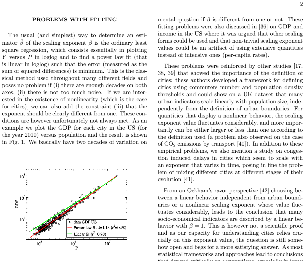
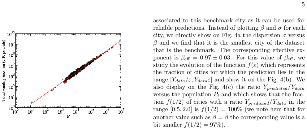
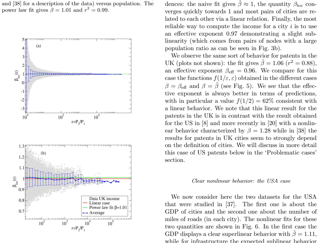
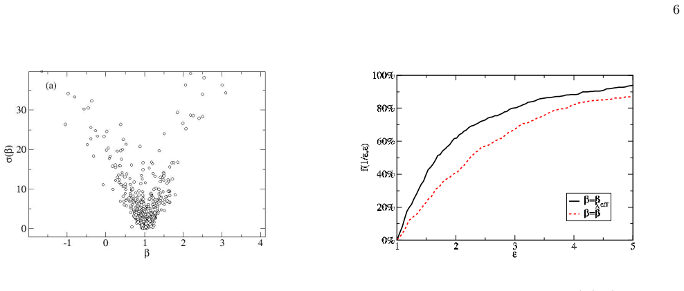
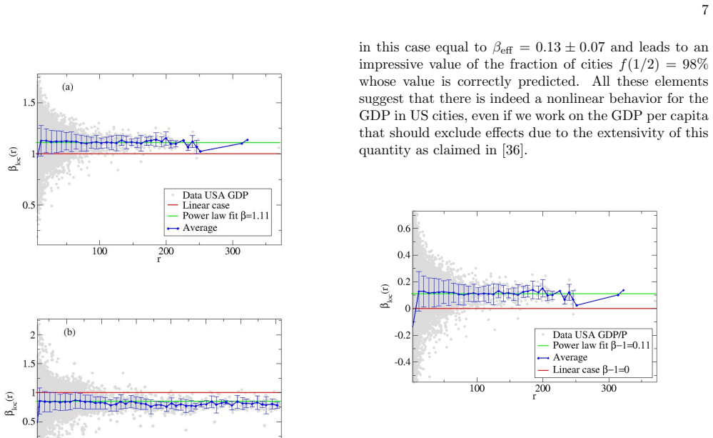
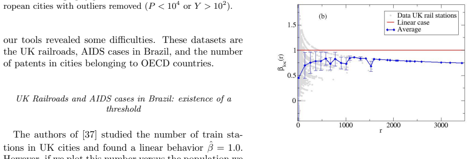
The central object is the local scaling exponent $\beta_{\mathrm{loc}}(i,j) = \log(Y_j/Y_i)/\log(P_j/P_i)$, viewed as a function of the size ratio $r$. It turns the global fitting problem into a family of pairwise comparisons, so the 'tomography plot' of $\beta_{\mathrm{loc}}$ versus $r$ shows convergence to a stable exponent when scaling holds, noise-dominated scatter for small $r$, and systematic features such as threshold hyperbolas or drift when the power-law form fails. The benchmark city is selected by minimising the variance of $\beta_{\mathrm{loc}}$ around its average, and that average is the effective exponent $\beta_{\mathrm{eff}}$ used for predictions via $Y(j) = Y(i_{\min})(P_j/P_{i_{\min}})^{\beta_{\mathrm{eff}}}$; the fraction $f(1/2)$ of cities predicted within a factor of two quantifies the value of the exponent.

What would settle it

Simulate a pure power law with constant prefactor and known $\beta$; the test is whether the tomography plot converges to that $\beta$ for large ratios. If it does not, or if a dataset with a known size-dependent prefactor still shows full convergence to one exponent, the central claim fails.

Watch

Extended reading notes

Core claim

The central claim is that the reliability of a scaling exponent can be assessed through local, ratio-based exponents instead of trusting a single regression. Defined as $\beta_{\mathrm{loc}} = \log(Y_2/Y_1)/\log(P_2/P_1)$, the local exponent is the slope of the chord between two cities in log-log space; plotting it against $r = P_2/P_1$ yields the 'tomography plot'. Under the scaling form $Y = a P^\beta$ with constant prefactor and moderate noise, $\beta_{\mathrm{loc}}$ converges to the true $\beta$ for large $r$ because the noise term is suppressed by $1/\log r$, and diverges for cities of nearly equal size. The paper defines the benchmark city as the one minimising the variance of $\beta_{\mathrm{loc}}$ over all other cities, and its mean local exponent $\beta_{\mathrm{eff}}$ as the best single exponent for prediction. Three necessary conditions are proposed for trusting a fitted exponent: convergence of $\beta_{\mathrm{loc}}$ to the fit, consistency of $\beta_{\mathrm{eff}}$ with the fit, and $f(1/2)$ at least 50%; otherwise the single-power-law form is rejected.

Load-bearing premise

The entire method assumes that the scaling law is exactly $Y = a P^\beta$ with a single constant prefactor $a$; if the prefactor varies systematically with population or region, the local exponent will absorb that variation and the effective exponent will not predict reliably.

Editorial extensions

If this is right

Scaling claims can be checked without assuming a particular noise model: genuine scaling requires $\beta_{\mathrm{loc}}$ to converge to the fitted exponent as the population ratio grows.
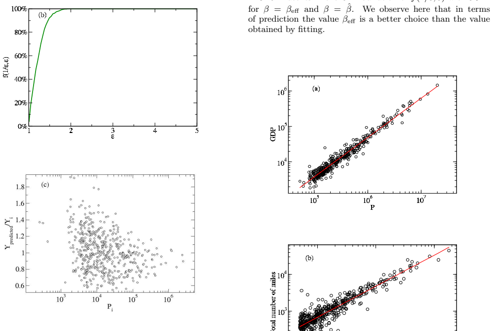
The effective exponent provides a direct prediction rule: with the benchmark city's $Y$ value and $\beta_{\mathrm{eff}}$, any other city's $Y$ can be estimated, and $f(1/2)$ gives its expected accuracy.
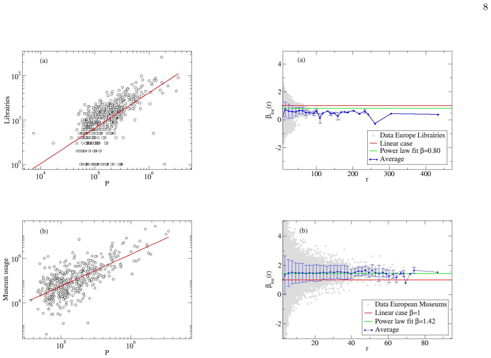
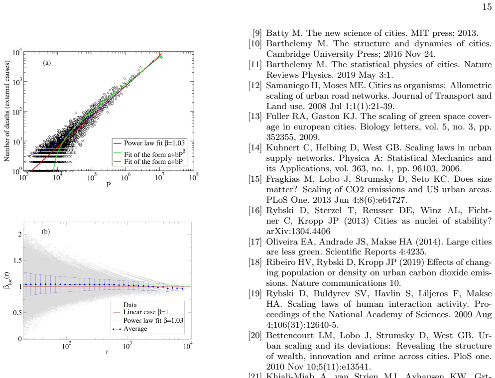
Cases that standard tools call inconclusive can be resolved: external-cause deaths in Brazil and cinema capacity in Europe come out linear, cinema usage in Europe superlinear with large fluctuations.
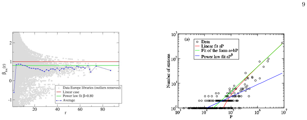
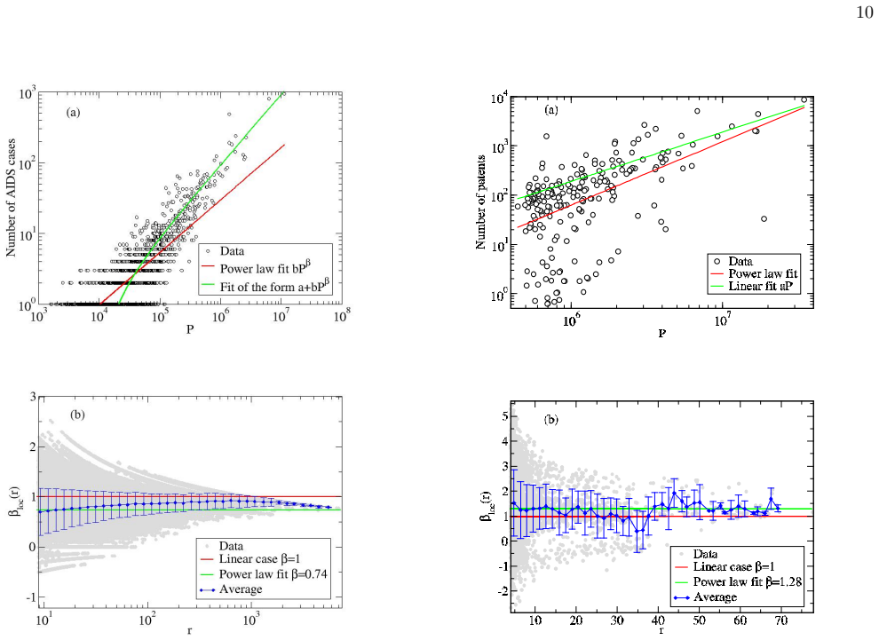
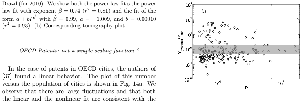
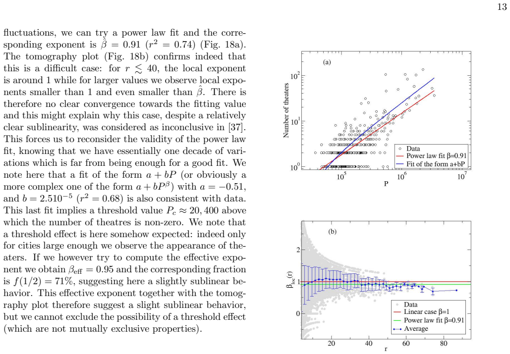
The method can reject the simple power-law form: UK railroads and Brazilian AIDS cases show threshold-like behaviour, and OECD patents are not described by a single exponent.
If the three necessary conditions fail, the fitted exponent should be abandoned; this gives a practical diagnostic beyond $r^2$ and $p$-values.

Reading between the lines

Editorial extensions of the paper, not claims the author makes directly.

A direct extension is to split city pairs into within-region and cross-region sets; if the effective exponent shifts between the two, the prefactor is not constant across regions and the single-exponent picture is misleading.
The decay of the noise envelope in the tomography plot is of order $1/\log r$, so the persistence of a gap between $\beta_{\mathrm{loc}}$ and the fitted exponent for large $r$ could be used as a quantitative test statistic for prefactor variation or wrong functional form.
The benchmark-city criterion (minimum variance of $\beta_{\mathrm{loc}}$) is one choice among many; testing sensitivity of $\beta_{\mathrm{eff}}$ to alternative criteria (e.g., the city closest to the regression line) would show how much of the conclusion is carried by the selection rule.
Because $\beta_{\mathrm{loc}}(r)$ is effectively a chord slope in log-log space, comparing its spectrum across $r$ ranges parallels the multiscaling analysis used in growth kinetics, suggesting a way to look for a continuum of exponents rather than a single one.

Share X Bluesky LinkedIn Reddit HN

Signed reviews

No signed human review yet.

Editorial analysis

A structured set of objections, weighed in public.

Desk editor's note, referee report, and a circularity audit.

Desk Editor's Note

read the letter

The core idea here is simple and genuinely useful: instead of fitting a global exponent, look at the local log-log slope between every pair of points and plot it against the size ratio. That tomography plot gives you a cheap visual check of whether a single scaling exponent is plausible, and it correctly flags cases where the standard fit is hiding something. The benchmark-city effective exponent, though, is a softer product.

The local exponent is elementary — it's just a chord slope in log-log space, and the paper acknowledges the connection to multiscaling. What's new is the packaging: the tomography plot, the benchmark-city minimization of the variance of beta_loc, and the f(1/2) accuracy fraction. Applied to the Leitao et al. datasets, these tools do what they promise: they confirm the clean cases (US GDP, roads), expose problems (UK rail stations, OECD patents), and give a plausible reading of some inconclusive cases. The writing is clear and the algebra in Eqs. 3-7 is correct.

The soft spots are in the claims around beta_eff. It is selected by minimizing the variance on the full dataset, and f(1/2) is then reported on the same data. That is in-sample fit quality, not predictive reliability. The paper says beta_eff lets you 'reliably' compute other cities' properties, but no out-of-sample test supports that word. The three necessary conditions in the Discussion are internal-consistency filters: if the prefactor varies systematically with P, beta_loc and the OLS fit will both converge to the same composite exponent, all three conditions pass, and the exponent is still not a stable predictor across regimes. The paper itself comes close to saying this for OECD patents. The threshold fits (a + bP) are also exploratory — extra parameters with comparable R^2 — and I read them as suggestive, not conclusive.

None of this sinks the paper. The descriptive diagnostic is solid and it is honestly presented. What needs fixing is the language of prediction and reliability. A referee should ask for an out-of-sample split or a careful restatement of beta_eff as a descriptive summary. My own verdict: conditional, but worth taking seriously.

Who is this for? Anyone working on urban scaling or other scaling data who wants a quick visual sanity check beyond a fitted line. It is a useful paper for that audience, and it deserves a serious referee. I would probably not cite it in my own work, but I would bring it to reading group.

Referee Report

3 major / 5 minor

Summary. The paper proposes a set of descriptive tools for studying scaling laws Y ~ P^β without relying on a regression fit. It defines a local exponent β_loc(i,j) = log(Y_j/Y_i)/log(P_j/P_i) for every pair of cities and plots this quantity against the population ratio r, calling the result a 'tomography plot'. It then defines an effective exponent β_eff as the mean local exponent of the benchmark city that minimizes the variance of β_loc, and claims that this exponent can be used to 'reliably' predict the properties of other cities through Eq. (12). The manuscript also proposes three necessary conditions for trusting a fitted exponent β_hat: convergence of β_loc toward β_hat, consistency of β_eff with β_hat, and a fraction f(1/2) of at least 50% of correctly predicted cities. These tools are applied to several urban datasets, showing cases where the method confirms standard fits, cases where it suggests threshold effects, and cases where it indicates that no simple single-exponent scaling holds.

Significance. If the proposed diagnostics are valid, they provide a simple and visually appealing complement to regression-based scaling analyses, with practical value for distinguishing linear, superlinear, and sublinear behavior in noisy, short-range city data. The algebraic derivation of the local exponent and its behavior under multiplicative noise (Eqs. 3-7) is sound and clearly explained. The application to multiple real datasets is a strength, and the paper honestly reports cases where its own diagnostics weaken previously drawn conclusions, such as the European libraries case. However, the central predictive claim is currently supported only by in-sample measures, and the proposed 'necessary conditions' are not logically necessary for the assumed scaling form. These issues do not invalidate the descriptive utility of the tomography plot, but they do require substantial revision of the reliability claims before the method can be recommended for practical prediction.

major comments (3)

[Section 3, Eqs. (10)-(12) and (14)-(15)] The effective exponent β_eff is selected by minimizing the variance σ^2(i) over all cities in the dataset, and the quality metric f(1/2) is evaluated on the same cities used for the selection. Consequently, the reported f(1/2) values measure in-sample fit quality, not predictive reliability for other cities. The text's claim that Eq. (12) allows computing 'reliably' properties of other cities needs support from an out-of-sample evaluation, such as a train/test split or leave-one-city-out cross-validation; this is currently absent.
[Discussion, conditions (i)-(iii)] The three proposed necessary conditions are not necessary for the scaling form Eq. (1) to be correct with a constant prefactor. In the multiplicative-noise model used in Eq. (4), exact scaling with large noise can produce f(1/2) < 50%, so condition (iii) is not necessary. Conversely, all three conditions can hold when Eq. (1) is violated by a systematically varying prefactor: if ln a = c ln P, both β_loc and the OLS fit converge to β + c, and β_eff will be consistent with that value, yet the constant-prefactor scaling form is false. The conditions are internal consistency checks among estimators, not tests of the scaling assumption, and the statement that failure of these conditions 'safely' rejects β_hat is not justified.
[Problematic cases, Figs. 12, 13, 15] The threshold interpretations for UK railroads, AIDS cases in Brazil, and US patents are supported mainly by comparing R^2 values of power-law fits and fits with one or two additional parameters, e.g., r2=0.98 versus 0.76 for railroads, and r2=0.93 versus 0.81 for AIDS. Because the threshold models have more parameters, these R^2 differences do not by themselves establish that the scaling form is inadequate. A model-comparison criterion that penalizes complexity (AIC/BIC or a likelihood-ratio test) is needed to substantiate the paper's threshold-related conclusions.

minor comments (5)

[Section 3, Eq. (4)] The multiplicative-noise model Y2 = Y1 r^β (1+η) is introduced without stating the support of η; the expansion log(1+η) requires η > -1, and the phrase 'when the noise is not too large' should be made quantitative.
[Discussion, condition (i) and Figs. 3, 7] The claimed convergence of β_loc toward β_hat is assessed visually from tomography plots, with no formal convergence statistic; a quantitative criterion (e.g., a threshold on the deviation of the binned average from β_hat) would make the first necessary condition testable.
[Fig. 13 caption] The caption contains a duplicated phrase: 'We show both the power law ﬁt s the power law ﬁt with exponent...', which should be corrected.
[Table II] The quantity r^2 is used throughout but never defined; stating that it is the coefficient of determination in log-log space would clarify the comparisons.
[Section 3, Eq. (13)] In the definition of SAMIs, the reference quantity Y0 is not defined; please specify what Y0 represents (e.g., the prefactor from the regression or a baseline city value).

Circularity Check

1 steps flagged · score 6.0 of 10

Reliability of β_eff is an in-sample fit: f(1/2) and consistency checks are computed on the same data used to estimate β_eff, so the predictive claim reduces to goodness-of-fit.

fitted input called prediction [Section 3, 'Identifying a benchmark city and defining an effective exponent', Eqs. (9)-(15); Discussion necessary conditions]
"This city can then serves as a benchmark in the sense that we can then use it for computing ‘reliably’ properties of other cities through the formula Y (j) =Y (imin)(Pj/Pimin)^βeff (12) and justiﬁes the denomination ‘eﬀective exponent’ as it can be used for practical predictions. ... We will systematically give the value of f(1/2) for ε2 = 2 as it gives a good idea of the accuracy of the prediction computed with βeﬀ."

βeff is defined as the average local exponent ⟨βloc(imin)⟩ computed from all pairs in the dataset, and the benchmark is selected as the city minimizing σ²(i) on that same dataset. The 'prediction' in Eq. (15) is then just Y(imin)(P/Pimin)^βeff, a one-parameter reconstruction of the same Y values used to estimate βeff; f(1/2) counts how many of these in-sample reconstructions fall within a factor of two of the actual data. No train/test split or cross-validation is performed. Thus the reported 'reliability' and 'accuracy of the prediction' are in-sample goodness-of-fit measures of a parameter fitted to the same data, not independent predictions.

full rationale

The paper's core mathematical construction — the local exponent βloc = log(Y2/Y1)/log(P2/P1), the tomography plot, and the benchmark defined by minimizing σ²(i) — is internally well-defined and not circular: βloc is a ratio of measured quantities, and βeff is an average of those ratios. The circularity enters specifically when the paper labels the resulting in-sample reconstruction a 'reliable' prediction. Since βeff and Y(imin) are estimated from the full dataset, Eq. (15) merely rearranges the same data, and f(1/2) records how well that one-parameter rearrangement fits the data it was built from. The Discussion's three necessary conditions are also internal-consistency checks (βloc vs β_hat, βeff vs β_hat, f(1/2)≥50%) and would not detect a misspecified prefactor that varies systematically with P, because both the local-exponent average and the OLS fit would track the same composite exponent. No self-citation is load-bearing in the derivation; the problem is the conflation of in-sample fit with predictive reliability. The score 6 reflects this partial circularity of the practical prediction claim, not of the mathematical definitions.

Assumptions & free parameters 3 free parameters · 4 assumptions · 0 invented entities

The method itself has few free parameters, but its empirical interpretations rely on fitted thresholds and an ad hoc reliability criterion. The central mathematical assumption is a constant prefactor in the scaling law, which is known to be questionable for urban data.

free parameters (3)

beta_eff (effective exponent) = varies by dataset (e.g., 0.966, 1.13, 0.17, 1.43)
Chosen as the average local exponent around the benchmark city; the predictive claim depends on this data-derived value.
Threshold population Pc = 30084 (UK railroads), 10090 (AIDS Brazil), 10500 (US patents), 20400 (theatres)
Fitted from a+bP or a+bP^beta models and used to argue for threshold effects.
f(1/2) criterion threshold = 0.5
Ad hoc rule proposed in the Discussion to decide trustworthiness of beta_hat.

assumptions (4)

domain assumption Scaling relation Y = a P^beta holds with a constant prefactor a.
Equation (1); the method's interpretation of beta_loc convergence relies on this.
ad hoc to paper Multiplicative noise model Y2 = Y1 r^beta (1+eta).
Equation (4) in Section 3; the convergence of beta_loc for large r is derived under this assumption.
domain assumption Cities are independent observations drawn from a single scaling law.
The benchmark city and effective exponent treat all cities as exchangeable, which fails for OECD patents.
domain assumption Standard statistical methods of [37] are correct as a baseline.
The paper uses [37] conclusions as reference labels for comparison.

how reviews work

0 comments

Cite this review

Pith. "Pith review of Tomography of scaling." pith.science (2026). https://pith.science/paper/R473FRPA

@misc{pith2026190811549,
  author       = {Pith},
  title        = {Pith review of: Tomography of scaling},
  year         = {2026},
  howpublished = {\url{https://pith.science/paper/R473FRPA}},
  note         = {Machine review of arXiv:1908.11549}
}

abstract

Scaling describes how a given quantity $Y$ that characterizes a system varies with its size $P$. For most complex systems it is of the form $Y\sim P^\beta$ with a nontrivial value of the exponent $\beta$, usually determined by regression methods. The presence of noise can make it difficult to conclude about the existence of a non-linear behavior with $\beta\neq 1$ and we propose here to circumvent fitting problems by investigating how two different systems of sizes $P_1$ and $P_2$ are related to each other. This leads us to define a local scaling exponent $\beta_{\mathrm{loc}}$ that we study versus the ratio $P_2/P_1$ and provides some sort of `tomography scan' of scaling across different values of the size ratio, allowing us to assess the relevance of nonlinearity in the system and to identify an effective exponent that minimizes the error for predicting the value of $Y$. We illustrate this method on various real-world datasets for cities and show that our method reinforces in some cases the standard analysis, but is also able to provide new insights in inconclusive cases and to detect problems in the scaling form such as the absence of a single scaling exponent or the presence of threshold effects.

Figures

Figures reproduced from arXiv: 1908.11549 by the authors.

**Figure 2.** FIG. 2: Total weekly income for cities in the UK (see [37] [PITH_FULL_IMAGE:figures/full_fig_p005_2.png] view at source ↗

**Figure 3.** FIG. 3: (a) ‘Tomography plot’ for the total weekly income [PITH_FULL_IMAGE:figures/full_fig_p005_3.png] view at source ↗

Figures from the paper (13 more)

**Figure 5.** Figure 5: FIG. 5: Patents in the UK: Variation of [PITH_FULL_IMAGE:figures/full_fig_p006_5.png]

**Figure 4.** Figure 4: FIG. 4: (a) Dispersion [PITH_FULL_IMAGE:figures/full_fig_p006_4.png]

**Figure 8.** Figure 8: FIG. 8: Tomography plot for the GDP per capita for US cities [PITH_FULL_IMAGE:figures/full_fig_p007_8.png]

**Figure 9.** Figure 9: FIG. 9: (a) Number of libraries in European cities (2011). [PITH_FULL_IMAGE:figures/full_fig_p008_9.png]

**Figure 10.** Figure 10: FIG. 10: Tomography plots for (a) the number of libraries [PITH_FULL_IMAGE:figures/full_fig_p008_10.png]

**Figure 11.** Figure 11: FIG. 11: Tomography plot for the number of libraries in Eu [PITH_FULL_IMAGE:figures/full_fig_p009_11.png]

**Figure 12.** Figure 12: FIG. 12: (a) Number of rail stations vs. population in UK [PITH_FULL_IMAGE:figures/full_fig_p009_12.png]

**Figure 13.** Figure 13: FIG. 13: (a) Number of AIDS cases versus city population in [PITH_FULL_IMAGE:figures/full_fig_p010_13.png]

**Figure 14.** Figure 14: FIG. 14: (a) Number of patents vs. population for cities in [PITH_FULL_IMAGE:figures/full_fig_p010_14.png]

**Figure 15.** Figure 15: FIG. 15: (a) Number of patents versus population for US [PITH_FULL_IMAGE:figures/full_fig_p011_15.png]

**Figure 17.** Figure 17: FIG. 17: Cinema usage in European cities for the year 2011. [PITH_FULL_IMAGE:figures/full_fig_p012_17.png]

**Figure 18.** Figure 18: FIG. 18: (a) Number of theaters in European cities versus [PITH_FULL_IMAGE:figures/full_fig_p013_18.png]

**Figure 19.** Figure 19: FIG. 19: Death by external causes in Brazil (year 2010). [PITH_FULL_IMAGE:figures/full_fig_p015_19.png]

Discussion (0). Continue with ORCID to comment.

Reference graph

Works this paper leans on

46 extracted references · 43 canonical work pages

[1]

Body size and metabolism

Kleiber M. Body size and metabolism. Hilgardia, Vol. 6, no 11, 1932

work page 1932
[2]

Body size and metabolic rate

Kleiber M. Body size and metabolic rate. Physiological reviews. 1947 Oct 1;27(4):511-41

work page 1947
[3]

Scaling concepts in polymer physics

De Gennes PG, Gennes PG. Scaling concepts in polymer physics. Cornell university press; 1979

work page 1979
[4]

Lectures on phase transitions and the renormalization group

Goldenfeld N. Lectures on phase transitions and the renormalization group. Perseus Books Publishing, 1992

work page 1992
[5]

Barenblatt GI. Scaling. Cambridge University Press; 2003

work page 2003
[6]

A general model for the origin of allometric scaling laws in biology

West GB, Brown JH, Enquist BJ. A general model for the origin of allometric scaling laws in biology. Science. 1997 Apr 4;276(5309):122-6

work page 1997
[7]

Scaling laws and urban systems

Pumain, Denise. Scaling laws and urban systems. Work- ing paper SFI. (2004)

work page 2004
[8]

Growth, innovation, scaling, and the pace of life in cities

Bettencourt LM, Lobo J, Helbing D, Khnert C, West GB. Growth, innovation, scaling, and the pace of life in cities. Proc. Natl. Acad. Sci. (USA) 104(17):7301-6 (2007)

work page 2007

Show all 46 references

[9]

The new science of cities

Batty M. The new science of cities. MIT press; 2013

2013
[10]

The structure and dynamics of cities

Barthelemy M. The structure and dynamics of cities. Cambridge University Press; 2016 Nov 24

2016
[11]

The statistical physics of cities

Barthelemy M. The statistical physics of cities. Nature Reviews Physics. 2019 May 3:1

2019
[12]

Cities as organisms: Allometric scaling of urban road networks

Samaniego H, Moses ME. Cities as organisms: Allometric scaling of urban road networks. Journal of Transport and Land use. 2008 Jul 1;1(1):21-39

2008
[13]

The scaling of green space cover- age in european cities

Fuller RA, Gaston KJ. The scaling of green space cover- age in european cities. Biology letters, vol. 5, no. 3, pp. 352355, 2009

2009
[14]

Scaling laws in urban supply networks

Kuhnert C, Helbing D, West GB. Scaling laws in urban supply networks. Physica A: Statistical Mechanics and its Applications, vol. 363, no. 1, pp. 96103, 2006

2006
[15]

Does size matter? Scaling of CO2 emissions and US urban areas

Fragkias M, Lobo J, Strumsky D, Seto KC. Does size matter? Scaling of CO2 emissions and US urban areas. PLoS One. 2013 Jun 4;8(6):e64727

2013
[16]

Rybski D, Sterzel T, Reusser DE, Winz AL, Ficht- ner C, Kropp JP (2013) Cities as nuclei of stability? arXiv:1304.4406

2013 arXiv
[17]

Large cities are less green

Oliveira EA, Andrade JS, Makse HA (2014). Large cities are less green. Scientiﬁc Reports 4:4235

2014
[18]

Nature communications 10

Ribeiro HV, Rybski D, Kropp JP (2019) Eﬀects of chang- ing population or density on urban carbon dioxide emis- sions. Nature communications 10

2019
[19]

Scaling laws of human interaction activity

Rybski D, Buldyrev SV, Havlin S, Liljeros F, Makse HA. Scaling laws of human interaction activity. Pro- ceedings of the National Academy of Sciences. 2009 Aug 4;106(31):12640-5

2009
[20]

Ur- ban scaling and its deviations: Revealing the structure of wealth, innovation and crime across cities

Bettencourt LM, Lobo J, Strumsky D, West GB. Ur- ban scaling and its deviations: Revealing the structure of wealth, innovation and crime across cities. PloS one. 2010 Nov 10;5(11):e13541

2010
[21]

PLoS ONE 14 (6): e0218022

Khiali-Miab A, van Strien MJ, Axhausen KW, Grt- Regamey A (2019) Combining urban scaling and poly- centricity to explain socioeconomic status of urban re- gions. PLoS ONE 14 (6): e0218022

2019
[22]

2013 Distance to the scaling law: a useful approach for unveil- ing relationships between crime and urban metrics.PLoS ONE 8, e69580

Alves LGA, Ribeiro HV, Lenzi EK, Mendes RS. 2013 Distance to the scaling law: a useful approach for unveil- ing relationships between crime and urban metrics.PLoS ONE 8, e69580. (doi:10.1371/journal. pone.0069580)

2013 doi
[23]

Urban scaling and the production function for cities

Lobo J, Bettencourt LM, Strumsky D, West GB. Urban scaling and the production function for cities. PLoS One. 2013 Mar 27;8(3):e58407

2013
[24]

Invention in the city: Increasing returns to patenting as a scaling func- tion of metropolitan size

Bettencourt LM, Lobo J, Strumsky D. Invention in the city: Increasing returns to patenting as a scaling func- tion of metropolitan size. Research policy. 2007 Feb 1;36(1):107-20

2007
[25]

2014 On scaling of scientiﬁc knowledge production in U.S

Nomaler O, Frenken K, Heimeriks G. 2014 On scaling of scientiﬁc knowledge production in U.S. metropolitan areas.PLoS ONE 9, e110805. (doi:10.1371/journal.pone.0110805)

2014 doi
[26]

Rich and poor cities in europe

Strano E, Sood V. Rich and poor cities in europe. An ur- ban scaling approach to mapping the european economic transition. PloS one, vol. 11, no. 8, p. e0159465, 2016

2016
[27]

PloS one, 12:e0171609

Caminha C, Furtado V, Pequeno TH, Ponte C, Melo HP, Oliveira EA, Andrade Jr JS (2017) Human mobility in large cities as a proxy for crime. PloS one, 12:e0171609

2017
[28]

An evolutionary theory for interpreting urban scaling laws

Pumain D, Paulus F, Vacchiani-Marcuzzo C, Lobo J. An evolutionary theory for interpreting urban scaling laws. Cybergeo: European Journal of Geography. 2006 Jul 5

2006
[29]

The origins of scaling in cities

Bettencourt LM. The origins of scaling in cities. science. 2013 Jun 21;340(6139):1438-41

2013
[30]

2013 The hypothesis 16 of urban scaling: formalization, implications and chal- lenges

Bettencourt LMA, Lobo J, Youn H. 2013 The hypothesis 16 of urban scaling: formalization, implications and chal- lenges. arXiv:1301.5919

2013 arXiv
[31]

Modeling the polycentric tran- sition of cities

Louf R, Barthelemy M. Modeling the polycentric tran- sition of cities. Physical review letters. 2013 Nov 6;111(19):198702

2013
[32]

How congestion shapes cities: from mobility patterns to scaling

Louf R, Barthelemy M. How congestion shapes cities: from mobility patterns to scaling. Scientiﬁc reports. 2014 Jul 3;4:5561

2014
[33]

Critical factors for miti- gating car traﬃc in cities

Verbavatz V, Barthelemy M. Critical factors for miti- gating car traﬃc in cities. PLoS ONE 14(7): e0219559 (2019)

2019
[34]

How the geometry of cities ex- plains urban scaling laws and determines their exponents

Molinero C, Thurner S. How the geometry of cities ex- plains urban scaling laws and determines their exponents. arXiv:1908.0747

1908
[35]

Bureau of Economic Analysis: https://apps.bea.gov/ iTable/iTable.cfm?isuri=1&reqid=70&step=1#isuri= 1&reqid=70&step=1 (accessed 20.08.2019)

2019
[36]

Scaling and hierarchy in urban economies

Shalizi CR. Scaling and hierarchy in urban economies. arXiv preprint arXiv:1102.4101, 2011

2011 arXiv
[37]

The plot of this number versus the population of cities is shown in Fig

found a linear behavior. The plot of this number versus the population of cities is shown in Fig. 14a. We observe that there are large ﬂuctuations and that both the linear and the nonlinear ﬁt are consistent with the data (this is obviously due to the noise and the small numbe...

2005
[38]

and below for a discussion about this point). Empir- ical results for various quantities in cities were compiled for the ﬁrst time in [8] and provided evidence that many quantities follow the scaling relation Y =aPβ (1) where a is a prefactor and where the exponent β is in gen...

2011 arXiv
[39]

Is this scaling nonlinear? Royal Society open science

Leitao JC, Miotto JM, Gerlach M, Altmann EG. Is this scaling nonlinear? Royal Society open science. 2016 Jul 1;3(7):150649

2016
[40]

Constructing cities, deconstructing scaling laws

Arcaute E, Hatna E, Ferguson P, Youn H, Johansson A, Batty M. Constructing cities, deconstructing scaling laws. Journal of The Royal Society Interface. 2015 Jan 6;12(102):20140745

2015
[41]

Diverse cities or the systematic paradox of urban scaling laws

Cottineau C, Hatna E, Arcaute E, Batty M. Diverse cities or the systematic paradox of urban scaling laws. Comput- ers, environment and urban systems. 2017 May 1;63:80- 94

2017
[42]

Scaling: lost in the smog

Louf R, Barthelemy M. Scaling: lost in the smog. En- vironment and Planning B: Planning and Design. 2014 Oct;41(5):767-9

2014
[43]

From global scaling to the dynamics of individual cities

Depersin J, Barthelemy M. From global scaling to the dynamics of individual cities. Proceedings of the National Academy of Sciences. 2018 Mar 6;115(10):2317-22

2018
[44]

Philosophical writings

Ockham W. Philosophical writings. Hackett Publising 1990

1990
[45]

Complex Networks and Fundamental Ur- ban Processes

Bettencourt L. Complex Networks and Fundamental Ur- ban Processes. Mansueto Institute for Urban Innovation Research Paper. 2019 Jun 11(9)

2019
[46]

Multiscaling in Growth Kinetics

Coniglio A, Zannetti M. Multiscaling in Growth Kinetics. Europhys. Lett., 10 (6), pp. 575-580 (1989)

1989

Pith tools

Reviewed August 14, 2026 · model on record in the stance chip above.

[1] [1]

Body size and metabolism

Kleiber M. Body size and metabolism. Hilgardia, Vol. 6, no 11, 1932

work page 1932

[2] [2]

Body size and metabolic rate

Kleiber M. Body size and metabolic rate. Physiological reviews. 1947 Oct 1;27(4):511-41

work page 1947

[3] [3]

Scaling concepts in polymer physics

De Gennes PG, Gennes PG. Scaling concepts in polymer physics. Cornell university press; 1979

work page 1979

[4] [4]

Lectures on phase transitions and the renormalization group

Goldenfeld N. Lectures on phase transitions and the renormalization group. Perseus Books Publishing, 1992

work page 1992

[5] [5]

Barenblatt GI. Scaling. Cambridge University Press; 2003

work page 2003

[6] [6]

A general model for the origin of allometric scaling laws in biology

West GB, Brown JH, Enquist BJ. A general model for the origin of allometric scaling laws in biology. Science. 1997 Apr 4;276(5309):122-6

work page 1997

[7] [7]

Scaling laws and urban systems

Pumain, Denise. Scaling laws and urban systems. Work- ing paper SFI. (2004)

work page 2004

[8] [8]

Growth, innovation, scaling, and the pace of life in cities

Bettencourt LM, Lobo J, Helbing D, Khnert C, West GB. Growth, innovation, scaling, and the pace of life in cities. Proc. Natl. Acad. Sci. (USA) 104(17):7301-6 (2007)

work page 2007