Data-inspired simulation of AR 11158
Pith reviewed 2026-06-25 20:34 UTC · model grok-4.3
The pith
A data-driven simulation of AR 11158 forms a magnetic flux rope that erupts in an X-flare once parts of it reach decay index values above 1.5.
A machine-rendered reading of the paper's core claim, the machinery that carries it, and where it could break.
Core claim
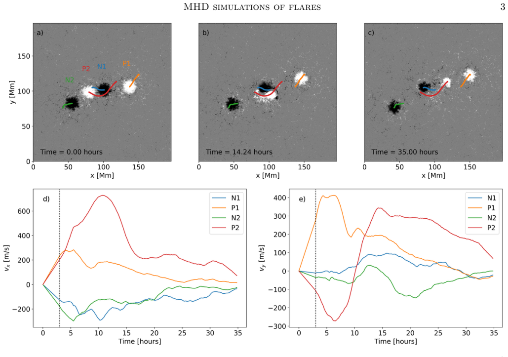
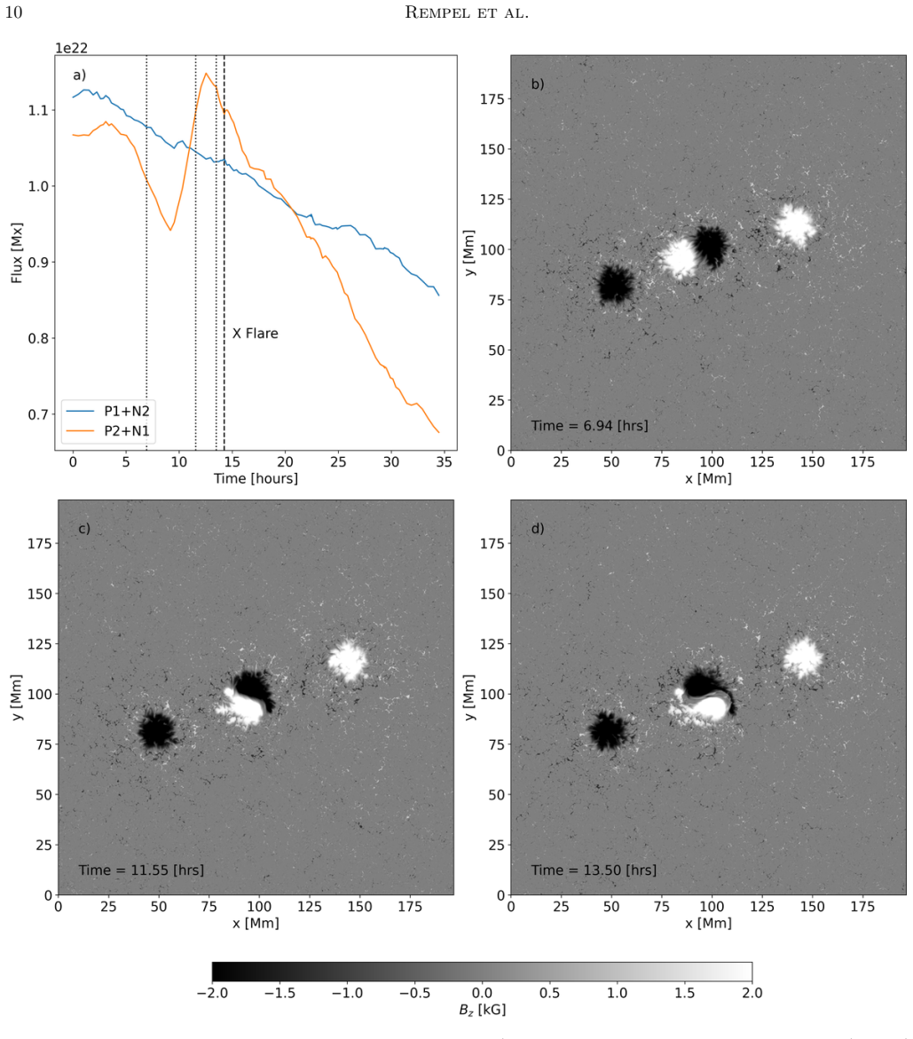
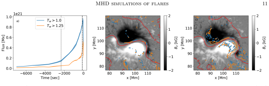
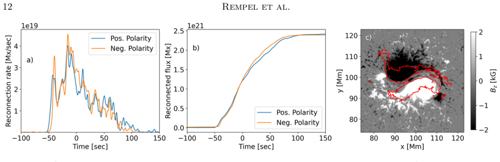
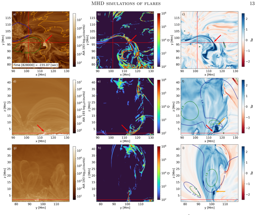
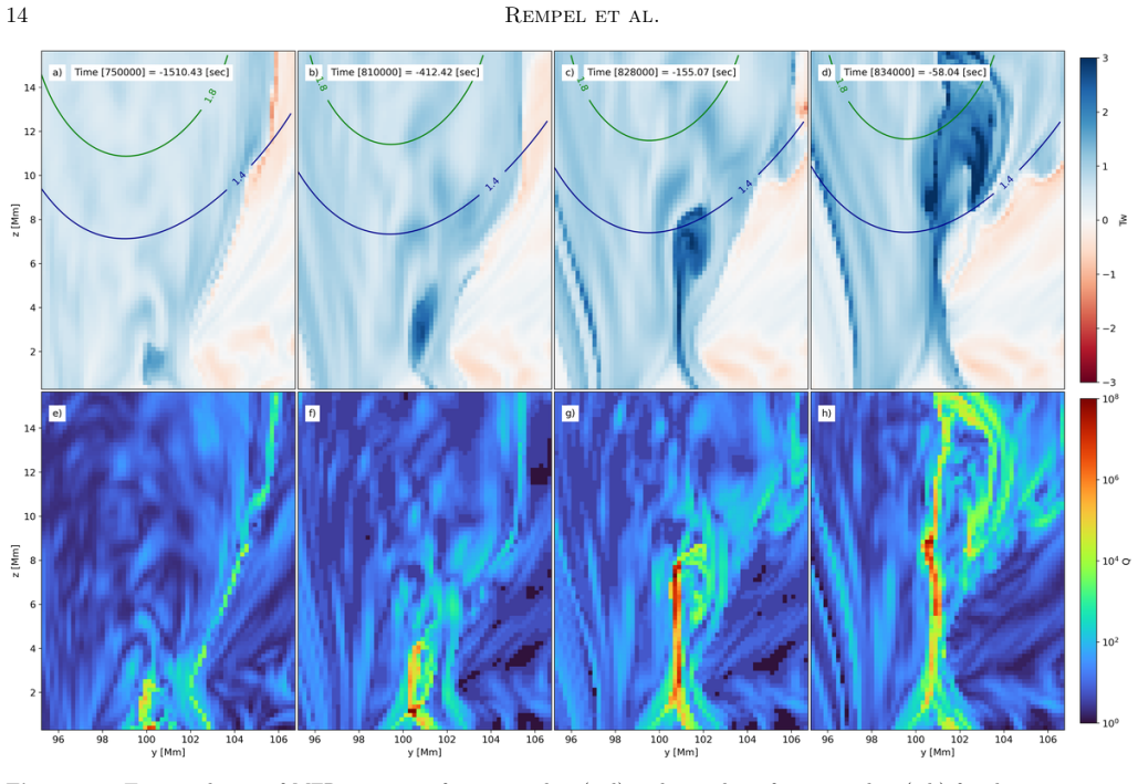
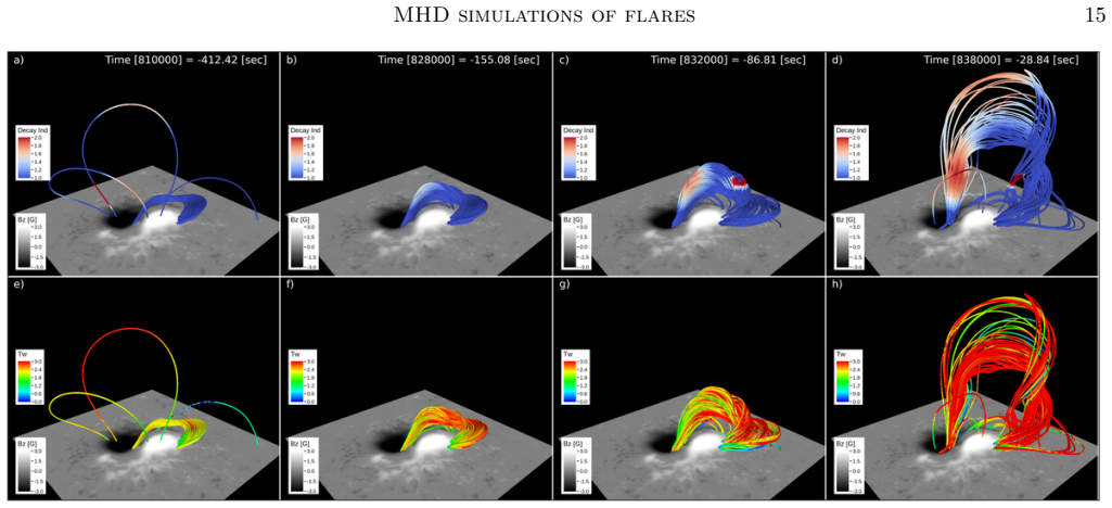
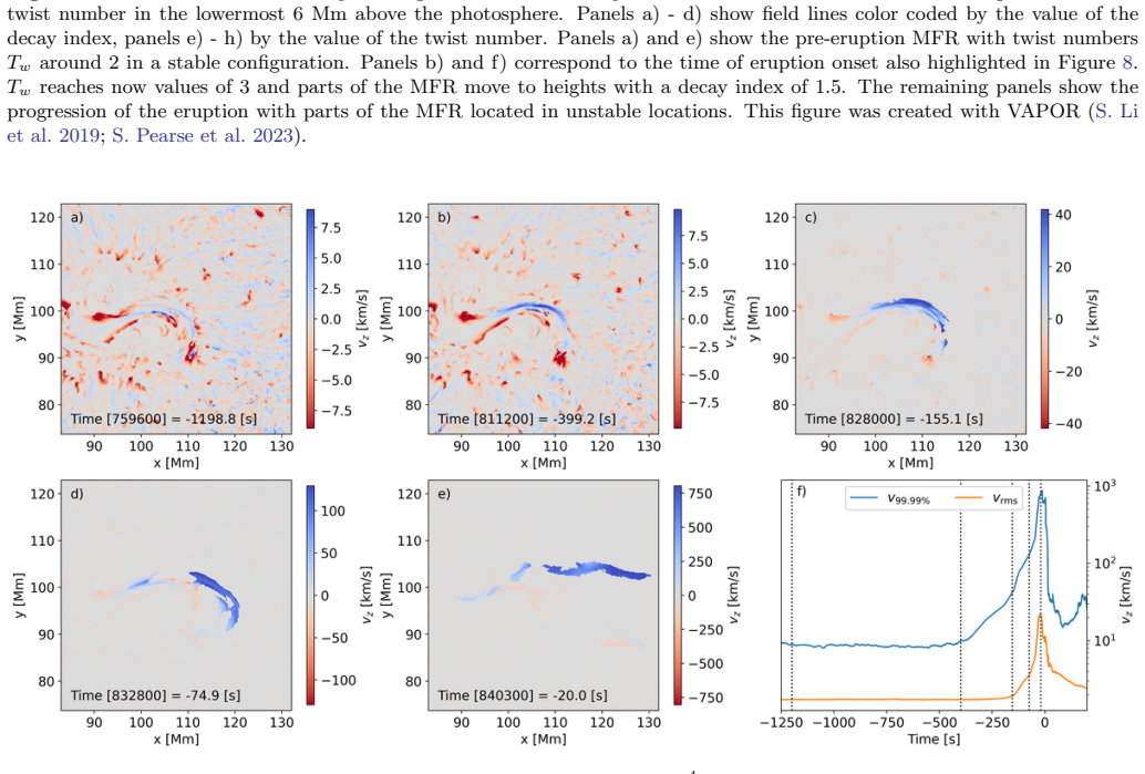
The simulation reproduces the observed timing and location of the X-flare by moving sunspots along measured paths, thereby forming a magnetic flux rope above the resulting collisional polarity inversion line. The rope rises and the flare initiates when portions of the rope enter regions with a decay index larger than 1.5. This sequence is presented as direct evidence that the torus instability governs the onset of the eruption in this active region.
What carries the argument
Data-inspired driving of sunspot motions along observed centroid positions within a quadrupolar magnetic configuration, which builds the collisional polarity inversion line and the overlying magnetic flux rope.
If this is right
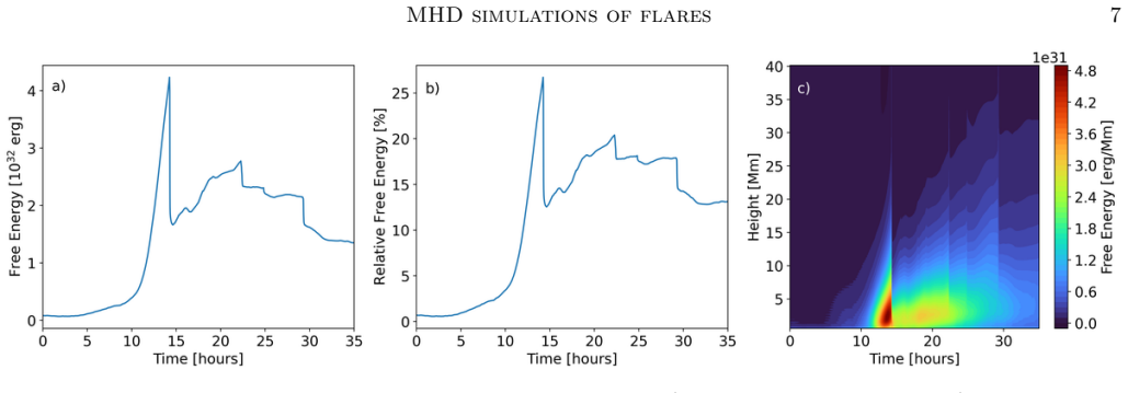
- Free energy in the corona exceeds 4 times 10 to the 32 erg, of which about 2 times 10 to the 32 erg is released during the X-flare and following smaller flares.
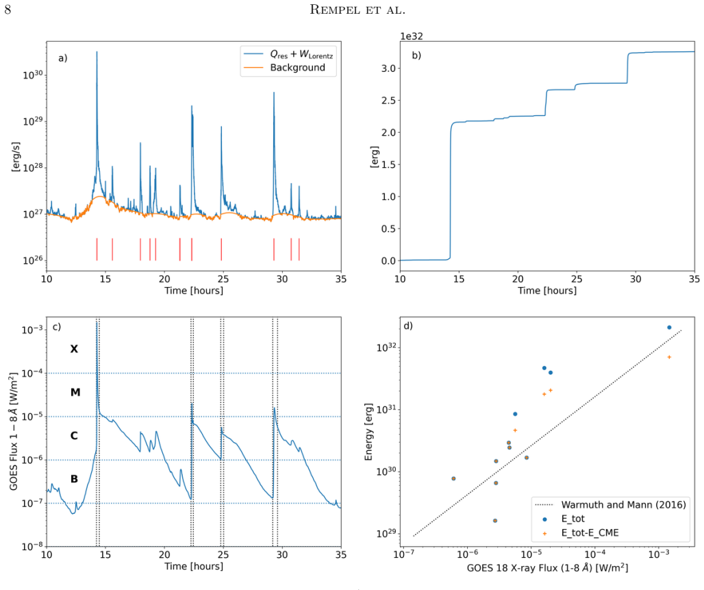
- The four strongest flares launch coronal mass ejections.
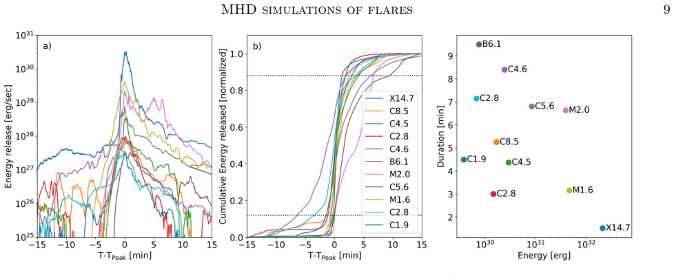
- Flare energies follow a trend with GOES X-ray flux similar to real events, but simulated durations lie at the short end of observed distributions.
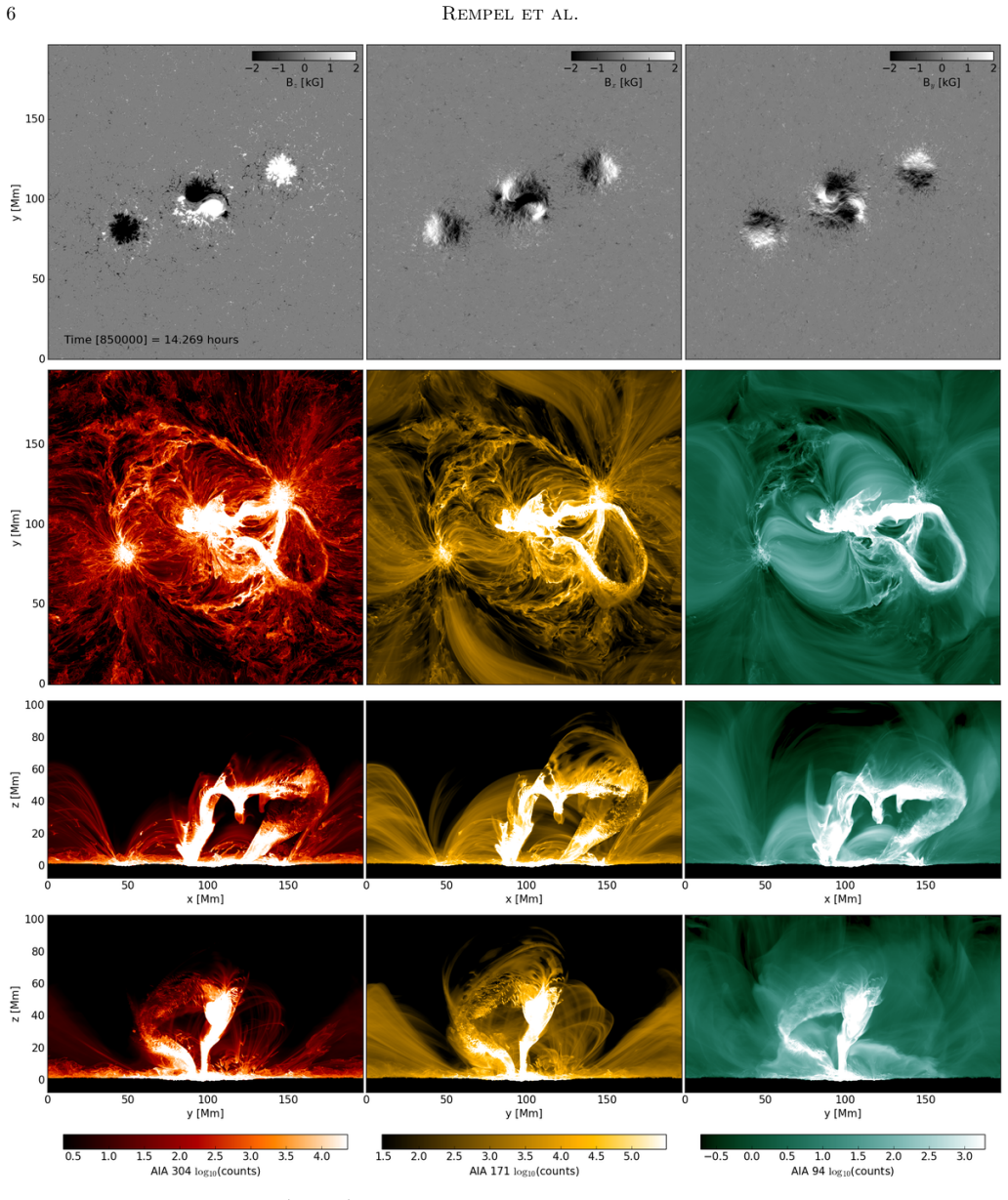
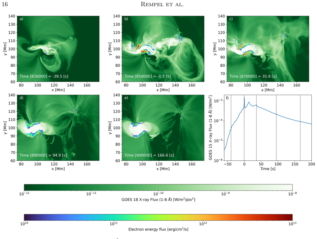
- Peak energy fluxes into the flare ribbons reach 10 to the 13 erg per square centimeter per second for the X-flare.
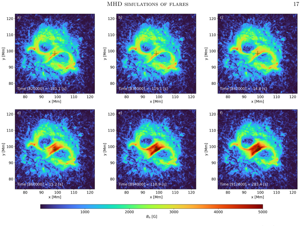
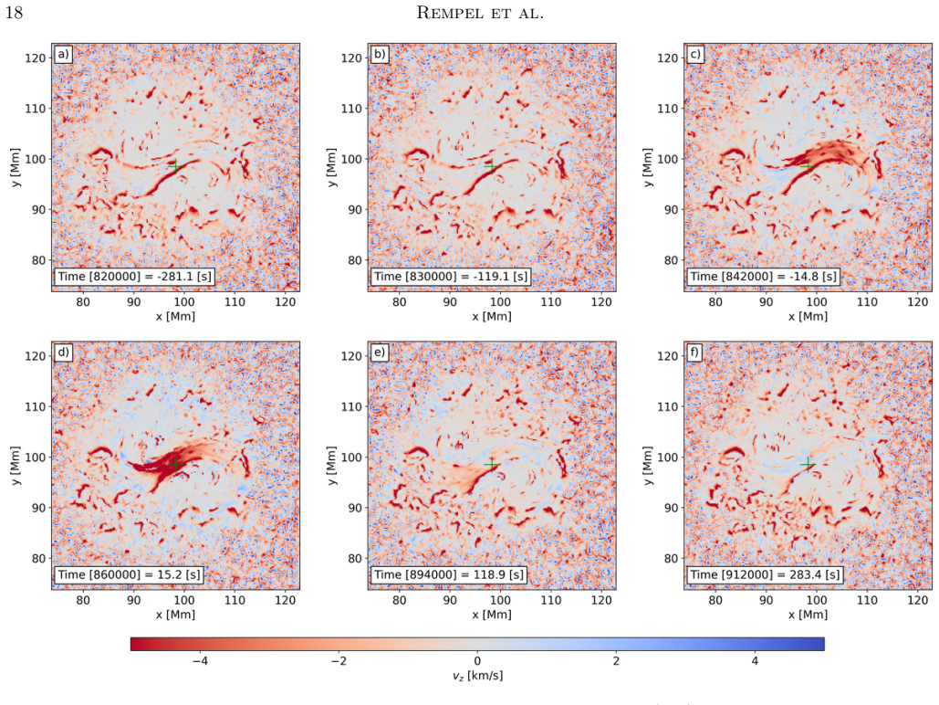
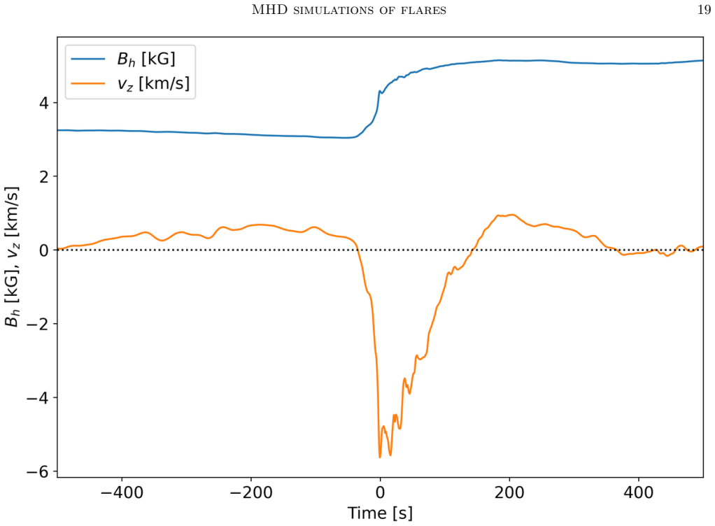
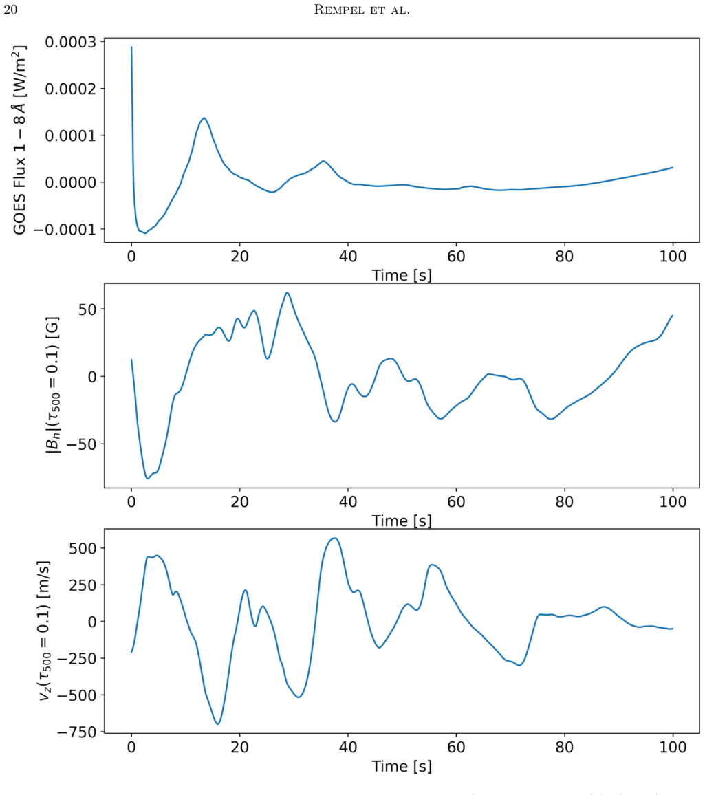
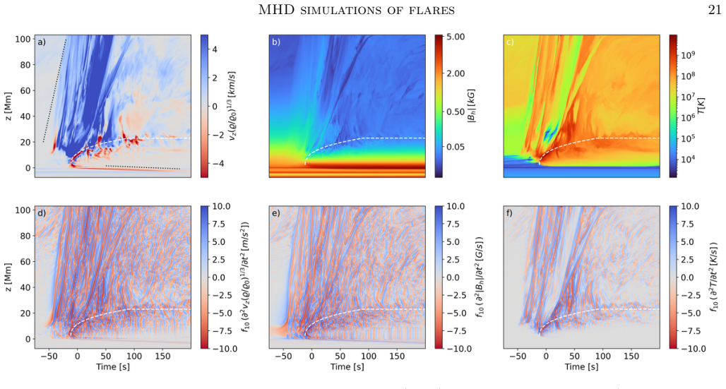
- The X-flare produces abrupt step-like increases in the horizontal photospheric field, launches a momentum pulse into the convection zone, and excites quasi-periodic pulsations throughout the coronal volume with periods ranging from sub-seconds to tens of seconds.
Where Pith is reading between the lines
- If the decay-index threshold reliably marks eruption onset in this setup, the same driving method could be applied to other active regions to test whether the torus instability criterion holds across multiple events.
- The short simulated flare durations imply that adding more realistic chromospheric radiation or resistivity might be needed to lengthen energy-release timescales toward observed values.
- The momentum pulse into the convection zone raises the possibility that the modeled eruption could produce detectable helioseismic signatures in the deeper solar interior.
Load-bearing premise
That displacing sunspots solely along the observed centroid tracks in a quadrupolar layout is sufficient to reproduce the real magnetic evolution, polarity inversion line formation, and coronal energy storage without extra unobserved flows or flux emergence.
What would settle it
High-cadence vector magnetograms of AR 11158 that show the actual photospheric field evolution or the timing of the collisional polarity inversion line diverging from the simulated sequence would falsify the claim that the chosen driving alone captures the essential buildup to eruption.
Figures
read the original abstract
We present a data-inspired simulation of NOAA active region AR 11158. We simulate the formation of a collisional polarity inversion line (cPIL) by moving sunspots in a quadrupolar configuration along the centroid positions extracted from AR 11158. This process builds up free energy in the corona exceeding $4\cdot 10^{32}$ erg, out of which about $2\cdot 10^{32}$ erg are released in a X-flare followed by a series of smaller flares in the B to M range. The 4 strongest flares are associated with coronal mass ejections. About 1-2 hours prior to the X-flare a magnetic flux rope (MFR) is forming above the cPIL. About 5 minutes before the flare an upflow at chromospheric heights indicates a rise of the MFR. The eruption starts when parts of the MFR enter regions with a decay index larger than 1.5, indicating that the flare initiation is consistent with the torus instability. Comparing the series of flares in this simulation to properties of observed flares, we find a comparable trend between flare energy and GOES X-ray flux, but flare duration falls into the short end of the observed solar distribution. As a consequence, energy fluxes into the flare ribbons can be substantial, reaching $10^{13}$ erg cm$^{-2}$ s$^{-1}$ for the simulated X-flare. The X-flare causes step-function like changes of the horizontal magnetic field in the photosphere, a propagation of a momentum pulse into the convection zone and quasi-periodic pulsations in the volume of the corona with periods from sub-seconds to multiple 10 seconds.
Editorial analysis
A structured set of objections, weighed in public.
Referee Report
Summary. The manuscript presents a data-inspired MHD simulation of AR 11158 in which sunspots in a quadrupolar configuration are displaced along observed centroid tracks to form a collisional polarity inversion line. This builds coronal free energy exceeding 4×10^32 erg, of which ~2×10^32 erg is released in an X-flare plus smaller B/M flares, four of which are associated with CMEs. A magnetic flux rope forms above the cPIL 1–2 h before the X-flare; an upflow appears ~5 min prior, and the eruption begins when portions of the MFR reach regions with external-field decay index n > 1.5, taken as evidence for the torus instability. Additional reported outcomes include step-like photospheric horizontal-field changes, a momentum pulse into the convection zone, and quasi-periodic pulsations with periods from sub-seconds to tens of seconds. Flare energy versus GOES flux follows an observed trend, though durations are at the short end of the distribution.
Significance. If the kinematic driving reproduces the essential magnetic evolution, the work supplies a concrete, observationally anchored example of free-energy storage and torus-instability onset, together with quantitative predictions for ribbon energy fluxes (up to 10^13 erg cm^{-2} s^{-1}) and coronal QPPs that are directly testable against multi-instrument data for AR 11158.
major comments (2)
- [Abstract] Abstract and driving-method description: the torus-instability conclusion (MFR reaching n > 1.5 at the observed flare time) is load-bearing, yet the simulation is driven exclusively by centroid displacements; no quantitative comparison of the simulated vector field or Poynting-flux time series against the full HMI vector-magnetogram sequence is reported, leaving the timing of the n > 1.5 crossing sensitive to any unobserved shear or emergence not captured by centroids.
- [Abstract / Results] Energy-buildup and release statements: the reported free-energy values (>4×10^32 erg stored, ~2×10^32 erg released) and the 1–2 h MFR-formation window lack accompanying convergence tests, resolution studies, or sensitivity runs with respect to the centroid-driving prescription, which directly affects the central claim that the simulated sequence matches the observed flare energetics.
minor comments (1)
- [Abstract] The abstract states that flare duration falls at the short end of the observed distribution but does not quantify how this affects the derived ribbon energy-flux values or their comparison to observations.
Simulated Author's Rebuttal
We appreciate the referee's thorough review and valuable feedback on our manuscript. Below we provide point-by-point responses to the major comments. We plan to make revisions to address the concerns raised regarding the driving method and the robustness of the energy calculations.
read point-by-point responses
-
Referee: [Abstract] Abstract and driving-method description: the torus-instability conclusion (MFR reaching n > 1.5 at the observed flare time) is load-bearing, yet the simulation is driven exclusively by centroid displacements; no quantitative comparison of the simulated vector field or Poynting-flux time series against the full HMI vector-magnetogram sequence is reported, leaving the timing of the n > 1.5 crossing sensitive to any unobserved shear or emergence not captured by centroids.
Authors: We acknowledge that our simulation is data-inspired and driven by sunspot centroid displacements extracted from observations, without performing a quantitative comparison to the full time series of HMI vector magnetograms. This approach captures the large-scale displacement but may miss additional contributions from shear flows or flux emergence not reflected in centroid motion. The timing of the n > 1.5 region being reached by the MFR is a direct outcome of the driving and aligns with the observed X-flare time. We will revise the abstract and add a discussion in the methods section to emphasize the limitations of the driving prescription and the potential sensitivity to unobserved magnetic evolution. No full vector comparison is feasible within the current framework without additional modeling techniques. revision: partial
-
Referee: [Abstract / Results] Energy-buildup and release statements: the reported free-energy values (>4×10^32 erg stored, ~2×10^32 erg released) and the 1–2 h MFR-formation window lack accompanying convergence tests, resolution studies, or sensitivity runs with respect to the centroid-driving prescription, which directly affects the central claim that the simulated sequence matches the observed flare energetics.
Authors: The reported free-energy storage and release, as well as the MFR formation window, are specific to the simulation parameters and driving used. We did not conduct explicit convergence tests, resolution studies, or sensitivity runs in the submitted manuscript, primarily due to the significant computational resources required for such MHD simulations. We will include additional text in the results section describing the numerical setup and resolution, and note that the energy values should be interpreted in the context of this specific model. We agree that sensitivity to the driving prescription is important and will discuss this as a caveat. revision: partial
Circularity Check
No significant circularity in data-driven simulation of AR 11158
full rationale
The paper performs a forward MHD simulation in which sunspot positions are prescribed directly from observed centroid tracks in a quadrupolar setup. Free-energy accumulation, MFR formation above the cPIL, the timing of its rise, and the moment when the external-field decay index exceeds 1.5 are all emergent outputs of the time-dependent evolution rather than quantities fitted or defined to match the target flare. The torus-instability threshold is an externally standard diagnostic applied to the simulated field; no self-citation, ansatz, or uniqueness theorem is invoked to force the result. The chain therefore remains independent of its inputs and receives the default non-circularity finding.
Axiom & Free-Parameter Ledger
axioms (1)
- domain assumption Standard ideal or resistive MHD equations govern the evolution of the solar corona and photosphere in the simulation.
Reference graph
Works this paper leans on
-
[1]
2026, Nature Astronomy, 10, 54, doi: 10.1038/s41550-025-02706-4
Ashfield, W., Polito, V., L¨ orinˇ c´ ık, J., et al. 2026, Nature Astronomy, 10, 54, doi: 10.1038/s41550-025-02706-4
-
[2]
Asplund, M., Grevesse, N., Sauval, A. J., & Scott, P. 2009, ARA&A, 47, 481, doi: 10.1146/annurev.astro.46.060407.145222
-
[3]
Aulanier, G., T¨ or¨ ok, T., D´ emoulin, P., & DeLuca, E. E. 2010, ApJ, 708, 314, doi: 10.1088/0004-637X/708/1/314
-
[4]
Barnes, G., Leka, K. D., Schumer, E. A., & Della-Rose, D. J. 2007, Space Weather, 5, S09002, doi: 10.1029/2007SW000317
-
[5]
2026, ApJ, 1000, 227, doi: 10.3847/1538-4357/ae47db
Chen, F. 2026, ApJ, 1000, 227, doi: 10.3847/1538-4357/ae47db
-
[6]
2022, ApJ, 937, 91, doi: 10.3847/1538-4357/ac8f95 24Rempel et al
Chen, F., Rempel, M., & Fan, Y. 2022, ApJ, 937, 91, doi: 10.3847/1538-4357/ac8f95 24Rempel et al
-
[7]
2023, ApJL, 954, L47, doi: 10.3847/2041-8213/acf3e4
Cheng, X., Xing, C., Aulanier, G., et al. 2023, ApJL, 954, L47, doi: 10.3847/2041-8213/acf3e4
-
[8]
2019, ApJ, 871, 67, doi: 10.3847/1538-4357/aaef30
Kazachenko, M. 2019, ApJ, 871, 67, doi: 10.3847/1538-4357/aaef30
-
[9]
Dere, K. P., Del Zanna, G., Young, P. R., & Landi, E. 2023, ApJS, 268, 52, doi: 10.3847/1538-4365/acec79
-
[10]
C., Lindsey, C., & Braun, D
Donea, A. C., Lindsey, C., & Braun, D. 1999, Romanian Astronomical Journal, 9, 71
1999
-
[11]
Fan, Y., Kazachenko, M. D., Afanasyev, A. N., & Fisher, G. H. 2024, ApJ, 975, 206, doi: 10.3847/1538-4357/ad7f53
-
[12]
2015, ApJ, 806, 79, doi: 10.1088/0004-637X/806/1/79
Fang, F., & Fan, Y. 2015, ApJ, 806, 79, doi: 10.1088/0004-637X/806/1/79
-
[13]
1992, PhyS, 46, 202, doi: 10.1088/0031-8949/46/3/002
Feldman, U. 1992, PhyS, 46, 202, doi: 10.1088/0031-8949/46/3/002
-
[14]
Fisher, G. H., Bercik, D. J., Welsch, B. T., & Hudson, H. S. 2012, SoPh, 277, 59, doi: 10.1007/s11207-011-9907-2
-
[15]
Gallagher, P. T., Moon, Y. J., & Wang, H. 2002, SoPh, 209, 171, doi: 10.1023/A:1020950221179
-
[16]
Georgoulis, M. K., & Rust, D. M. 2007, ApJL, 661, L109, doi: 10.1086/518718
-
[17]
2010, Physics of Plasmas, 17, 062104, doi: 10.1063/1.3420208
Huang, Y.-M., & Bhattacharjee, A. 2010, Physics of Plasmas, 17, 062104, doi: 10.1063/1.3420208
-
[18]
Hudson, H. S. 2000, ApJL, 531, L75, doi: 10.1086/312516
-
[19]
Irwin, A. W. 2012,, Astrophysics Source Code Library, record ascl:1211.002 http://ascl.net/1211.002
2012
-
[20]
2022, Nature Reviews Physics, 4, 263, doi: 10.1038/s42254-021-00419-x
Ji, H., Daughton, W., Jara-Almonte, J., et al. 2022, Nature Reviews Physics, 4, 263, doi: 10.1038/s42254-021-00419-x
-
[21]
Johnston, C. D., Hood, A. W., De Moortel, I., Pagano, P., & Howson, T. A. 2021, A&A, 654, A2, doi: 10.1051/0004-6361/202140987
-
[22]
Kazachenko, M. D., Lynch, B. J., Welsch, B. T., & Sun, X. 2017, ApJ, 845, 49, doi: 10.3847/1538-4357/aa7ed6
-
[23]
S., Polito, V., Xu, Y., & Allred, J
Kerr, G. S., Polito, V., Xu, Y., & Allred, J. C. 2024, ApJ, 970, 21, doi: 10.3847/1538-4357/ad47e1
-
[24]
2016, ApJ, 816, 88, doi: 10.3847/0004-637X/816/2/88
Kleint, L., Heinzel, P., Judge, P., & Krucker, S. 2016, ApJ, 816, 88, doi: 10.3847/0004-637X/816/2/88
-
[25]
Kliem, B., Lin, J., Forbes, T. G., Priest, E. R., & T¨ or¨ ok, T. 2014, ApJ, 789, 46, doi: 10.1088/0004-637X/789/1/46
-
[26]
2006, PhRvL, 96, 255002, doi: 10.1103/PhysRevLett.96.255002
Kliem, B., & T¨ or¨ ok, T. 2006, PhRvL, 96, 255002, doi: 10.1103/PhysRevLett.96.255002
-
[27]
Kosovichev, A. G. 2006, SoPh, 238, 1, doi: 10.1007/s11207-006-0190-6
-
[28]
2017, ApJ, 836, 12, doi: 10.3847/1538-4357/836/1/12
Carlsson, M. 2017, ApJ, 836, 12, doi: 10.3847/1538-4357/836/1/12
-
[29]
Kowalski, A. F., Hawley, S. L., Carlsson, M., et al. 2015, SoPh, 290, 3487, doi: 10.1007/s11207-015-0708-x K¨ unzel, H. 1960, Astronomische Nachrichten, 285, 271, doi: 10.1002/asna.19592850516
-
[30]
Kuridze, D., Mathioudakis, M., Sim˜ oes, P. J. A., et al. 2015, ApJ, 813, 125, doi: 10.1088/0004-637X/813/2/125
-
[31]
2019, Atmosphere, 10, 488, doi: 10.3390/atmos10090488
Li, S., Jaroszynski, S., Pearse, S., Orf, L., & Clyne, J. 2019, Atmosphere, 10, 488, doi: 10.3390/atmos10090488
-
[32]
Linton, M. G., Dahlburg, R. B., Fisher, G. H., & Longcope, D. W. 1998, ApJ, 507, 404, doi: 10.1086/306299
-
[33]
Linton, M. G., Fisher, G. H., Dahlburg, R. B., & Fan, Y. 1999, ApJ, 522, 1190, doi: 10.1086/307678
-
[34]
Sterling, A. C. 2026, ApJ, 1000, 270, doi: 10.3847/1538-4357/ae4d11
-
[35]
Neupert, W. M. 1968, ApJL, 153, L59, doi: 10.1086/180220
-
[36]
2023,, 3.8.1 Zenodo, doi: 10.5281/zenodo.7779648
Pearse, S., Li, S., Clyne, J., et al. 2023,, 3.8.1 Zenodo, doi: 10.5281/zenodo.7779648
-
[37]
Uitenbroek, H., & Scherrer, P. H. 2025, ApJS, 278, 55, doi: 10.3847/1538-4365/adcf9f
-
[38]
Petrie, G. J. D., & Sudol, J. J. 2010, ApJ, 724, 1218, doi: 10.1088/0004-637X/724/2/1218
-
[39]
Reep, J. W., & Knizhnik, K. J. 2019, ApJ, 874, 157, doi: 10.3847/1538-4357/ab0ae7
-
[40]
2012, ApJ, 750, 62, doi: 10.1088/0004-637X/750/1/62
Rempel, M. 2012, ApJ, 750, 62, doi: 10.1088/0004-637X/750/1/62
-
[41]
2014, ApJ, 789, 132, doi: 10.1088/0004-637X/789/2/132
Rempel, M. 2014, ApJ, 789, 132, doi: 10.1088/0004-637X/789/2/132
-
[42]
2015, ApJ, 814, 125, doi: 10.1088/0004-637X/814/2/125
Rempel, M. 2015, ApJ, 814, 125, doi: 10.1088/0004-637X/814/2/125
-
[43]
2017, ApJ, 834, 10, doi: 10.3847/1538-4357/834/1/10
Rempel, M. 2017, ApJ, 834, 10, doi: 10.3847/1538-4357/834/1/10
-
[44]
Rempel, M., Chintzoglou, G., Cheung, M. C. M., Fan, Y., & Kleint, L. 2023, ApJ, 955, 105, doi: 10.3847/1538-4357/aced4d
-
[45]
Schrijver, C. J. 2007, ApJL, 655, L117, doi: 10.1086/511857
-
[46]
Sudol, J. J., & Harvey, J. W. 2005, ApJ, 635, 647, doi: 10.1086/497361
-
[47]
Takasao, S., Fan, Y., Cheung, M. C. M., & Shibata, K. 2015, ApJ, 813, 112, doi: 10.1088/0004-637X/813/2/112
-
[48]
Tamburri, C. A., Kazachenko, M. D., & Kowalski, A. F. 2024, ApJ, 966, 94, doi: 10.3847/1538-4357/ad3047
-
[49]
2014, SoPh, 289, 3351, doi: 10.1007/s11207-014-0502-1
Toriumi, S., Iida, Y., Kusano, K., Bamba, Y., & Imada, S. 2014, SoPh, 289, 3351, doi: 10.1007/s11207-014-0502-1
-
[50]
2017, ApJ, 850, 39, doi: 10.3847/1538-4357/aa95c2
Toriumi, S., & Takasao, S. 2017, ApJ, 850, 39, doi: 10.3847/1538-4357/aa95c2
-
[51]
Uzdensky, D. A., Loureiro, N. F., & Schekochihin, A. A. 2010, PhRvL, 105, 235002, doi: 10.1103/PhysRevLett.105.235002
-
[52]
1992, SoPh, 140, 85, doi: 10.1007/BF00148431 MHD simulations of flares25
Wang, H. 1992, SoPh, 140, 85, doi: 10.1007/BF00148431 MHD simulations of flares25
-
[53]
2012, ApJL, 745, L17, doi: 10.1088/2041-8205/745/2/L17
Wang, S., Liu, C., Liu, R., et al. 2012, ApJL, 745, L17, doi: 10.1088/2041-8205/745/2/L17
-
[54]
2016, A&A, 588, A115, doi: 10.1051/0004-6361/201527474
Warmuth, A., & Mann, G. 2016, A&A, 588, A115, doi: 10.1051/0004-6361/201527474
-
[55]
Wright, E., Brown, C., Przybylski, D., et al. 2023, in Proceedings of the SC ’23 Workshops of the International Conference on High Performance Computing, Network, Storage, and Analysis, SC-W ’23 (New York, NY, USA: Association for Computing Machinery), 1929–1938, doi: 10.1145/3624062.3624606
-
[56]
Wright, E., Przybylski, D., Rempel, M., et al. 2021, in Proceedings of the Platform for Advanced Scientific Computing Conference, PASC ’21 (New York, NY, USA: Association for Computing Machinery), doi: 10.1145/3468267.3470576
-
[57]
2024, ApJ, 966, 70, doi: 10.3847/1538-4357/ad2ea9
Xing, C., Aulanier, G., Cheng, X., Xia, C., & Ding, M. 2024, ApJ, 966, 70, doi: 10.3847/1538-4357/ad2ea9
-
[58]
2022, ApJ, 937, 26, doi: 10.3847/1538-4357/ac8d61
Zhang, P., Chen, J., Liu, R., & Wang, C. 2022, ApJ, 937, 26, doi: 10.3847/1538-4357/ac8d61
-
[59]
Zimovets, I. V., McLaughlin, J. A., Srivastava, A. K., et al. 2021, SSRv, 217, 66, doi: 10.1007/s11214-021-00840-9
discussion (0)
Sign in with ORCID, Apple, or X to comment. Anyone can read and Pith papers without signing in.