The Augmented Tree Tensor Network Cookbook

Daniel Jaschke; Luka Pave\v{s}i\'c; Nora Reini\'c; Simone Montangero

REVIEW 2 major objections 6 minor 46 references

The Augmented Tree Tensor Network Cookbook

T0 review · 2 major / 6 minor · reviewed 2026-08-06 · deepseek-v4-flash

Challenge this review Re-run · record.json Download PDF Read on arXiv ↗ Review JSON

Pith's one-line read An augmented tree tensor network—a TTN with a layer of unitary disentanglers—gives higher ground-state accuracy than MPS or TTN at fixed computational resources for large 2D lattices near a quantum critical point.

desk verdict A genuinely useful aTTN implementation guide, but the headline benchmark advantage over TTN near criticality is not fully supported without convergence checks. read the letter →

arxiv 2507.21236 v1 pith:R4R5DQF2 submitted 2025-07-28 quant-ph

Nora Reinić , Luka Pavešić , Daniel Jaschke , Simone Montangero This is my paper · ORCID

classification quant-ph MSC 81-0882B80

keywords augmentedtreetensornetworkdisentanglermatrixproductstategroundsearchquantumIsingmodeltriangularHeisenbergbenchmark

verification ladder T0 review T1 audit T2 compute T3 formal

The pith

A machine-rendered reading of the paper's core claim, the machinery that carries it, and where it could break.

The reading

This paper is a practical guide that establishes when an augmented tree tensor network (aTTN) beats two standard tensor network ansätze, matrix product states (MPS) and tree tensor networks (TTN), for two-dimensional quantum lattice models. The aTTN is a TTN with a layer of two-site unitary gates, called disentanglers, placed on its physical links; the disentanglers absorb entanglement that would otherwise require a larger bond dimension. The authors present the full variational ground-state search algorithm, including a MERA-like disentangler optimization via singular value decomposition and the mapping of the Hamiltonian to an auxiliary one, and benchmark it on square-lattice Ising and triangular-lattice Heisenberg models up to $32\times 32$ spins. They find that the aTTN consistently lowers the ground-state energy at fixed bond dimension, with the largest gains near criticality, and that for large enough lattices it gives the best accuracy relative to runtime and memory, while keeping the same $O(m^3)$ memory scaling with bond dimension as the TTN.

What carries the argument

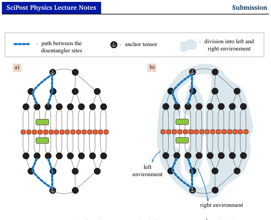
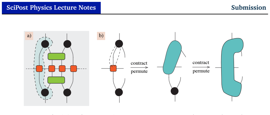
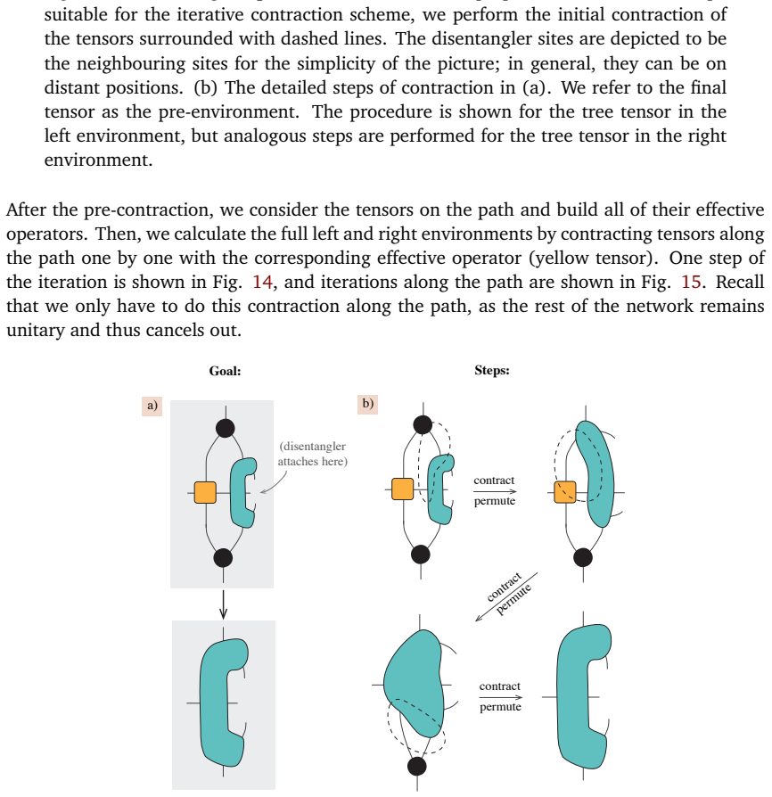
The augmented tree tensor network (aTTN): a tree tensor network whose lowest physical layer is preceded by a layer of two-site unitary gates (disentanglers), each attached to a pair of physical sites. The disentanglers absorb short-range entanglement and are optimized one at a time by freezing the conjugate gate, contracting the surrounding tensor network into a global environment $\Gamma_k$, and taking $u_k = -VU^\dagger$ from the singular value decomposition $\Gamma_k = U\sigma V^\dagger$, iterated to self-consistency. After the disentangler layer is found, the Hamiltonian is mapped to an auxiliary one, $H' = D(u)HD^\dagger(u)$, by contracting the disentanglers into the Hamiltonian's tensor-product-operator (TPO) terms, and a variational TTN sweep (DMRG) is run on the auxiliary Hamiltonian; measuring an observable proceeds the same way, by contracting the disentangler layer into the observable before evaluating it on the TTN. The TPO representation of the Hamiltonian is what lets each energy contribution be split into terms that touch a given disentangler and terms that do not.

What would settle it

Repeat the $32\times 32$ Ising benchmark at $h=3$ with many more disentangler-optimization sweeps and with random restarts, and compare the best aTTN energy at $m=160$ against the TTN at $m=400$; if the aTTN advantage shrinks or vanishes, the claimed advantage depends on the optimization stopping point rather than on the ansatz.

Watch

Extended reading notes

Core claim

The central claim is that appending one layer of unitary disentanglers to a tree tensor network improves the accuracy-to-cost tradeoff of ground-state searches in two dimensions, provided the lattice is large enough and the state is sufficiently entangled. In the $32\times 32$ square-lattice Ising model at transverse field $h=3$, near the critical point $h_c\approx 3.044$, the aTTN with bond dimension $m=160$ reaches lower energy densities than a TTN with $m=400$, and lower than the best MPS at $m=1200$, within the same memory budget. The advantage concentrates close to the critical point and grows with lattice size, because larger lattices allow more disentanglers and produce more long-range interactions that the disentanglers capture. For the triangular Heisenberg model the aTTN does not outperform TTN or MPS within the same resources, which the authors attribute to the larger number of Hamiltonian terms inflating the memory prefactor and to geometric restrictions that leave fewer viable disentangler positions. The memory cost of the aTTN scales with bond dimension $m$ as $O(m^3)$, the same as a TTN, with a constant prefactor about 6.5--10.9 times larger depending on model and size.

Load-bearing premise

The benchmark conclusions assume that the disentangler optimization converges to a sufficiently good disentangler layer within the fixed number of sweeps and iterations used; the paper does not analyze the convergence of that optimization.

Editorial extensions

If this is right

The aTTN gives lower ground-state energy than the TTN at every bond dimension tested for the $32\times 32$ Ising model near criticality.
For $32\times 32$ lattices near the critical point, the aTTN at $m=160$ beats both the TTN at $m=400$ and the best MPS within the same memory resources, while for $16\times 16$ lattices the MPS remains competitive.
The memory cost of the aTTN scales as $O(m^3)$, identical to the TTN, with a prefactor roughly 6.5--9.8 times larger for the Ising model and 8.7--10.9 times larger for the Heisenberg model.
Far from the critical point, where entanglement is low, a higher-bond-dimension TTN outperforms the aTTN at the same resource budget.
For the triangular Heisenberg model, the aTTN does not outperform TTN or MPS with the given resources; the authors identify the memory overhead of many enlarged Hamiltonian terms and the reduced number of allowed disentangler positions as the causes.

Reading between the lines

Editorial extensions of the paper, not claims the author makes directly.

The authors leave the compression of overlapping Hamiltonian TPO terms after disentangler contraction as future work; a concrete test of the paper's resource analysis would be to measure peak GPU memory before and after such a compression and check whether the aTTN's advantageous regime widens.
The empirical finding that one TTN-only sweep before disentangler optimization works best suggests the disentangler optimization can get trapped; a testable extension is to run multiple random restarts or a longer disentangler schedule to see whether the reported energies improve further.
Since the aTTN is a subclass of MERA with one disentangler layer, the cookbook's measurement recipes should carry over to other single-layer MERA-inspired ansätze; a natural test is to apply the same contraction strategy to a two-dimensional MERA with only the bottom layer disentangled.
The authors name time evolution as the next step; a direct benchmark would compare aTTN time evolution against MPS TDVP for a quench in the 2D transverse-field Ising model, looking for the same near-critical advantage seen in ground-state energies.

Share X Bluesky LinkedIn Reddit HN

Editorial analysis

A structured set of objections, weighed in public.

Desk editor's note, referee report, and a circularity audit.

Desk Editor's Note

read the letter

Dear Colleague,

The aTTN cookbook is a genuinely useful implementation guide, and the benchmark data are a real step forward. But the headline comparison—aTTN outperforming TTN at fixed resources on 32×32 Ising near criticality—rests on a fixed 30-sweep cutoff with no convergence check for the TTN at h=3. So I'd treat the advantage as plausible but not nailed down.

What's new: the ansatz itself is from Refs. [25,26], but this paper contributes a detailed recipe for the environment contractions, the disentangler optimization (both MERA-like and gradient descent), the TPO contraction logic, and a measurement protocol. The complexity analysis is clear, and the open-source implementation in Quantum TEA plus Zenodo data make it reproducible. The benchmarks cover two models and multiple system sizes, and the authors honestly report the triangular Heisenberg case where aTTN does not win. That negative result is a credit to them.

The main soft spot is convergence. All ground state searches stop at 30 DMRG sweeps, and the only convergence plot (Fig. 27b) is for TTN at h=1, in the bulk. At h=3, near criticality, the m=400 TTN may well need more sweeps than the m=160 aTTN to converge, and the differences in Fig. 29 could then be a convergence-speed effect rather than an advantage of the ansatz. The paper should either show energy versus sweep count for the compared bond dimensions at h=3, or at least argue why 30 sweeps is sufficient there. Also missing is the number of self-consistent iterations N_i in the MERA-like disentangler optimization for the benchmarks; without that, the aTTN results themselves are not fully characterized, though that would bias against the aTTN rather than for it.

These are fixable with additional data, not conceptual flaws. The computational complexity analysis holds up, and the algorithm descriptions match the cited literature.

For a tensor network practitioner implementing aTTNs or planning benchmarks, this is a valuable reference. The measurement chapter and the disentangler positioning discussion alone are worth the read. The central benchmark claim should be treated as provisional until the convergence checks are added.

I'd send it to peer review—it deserves a serious referee—with the main request being additional convergence data for the key comparison.

Referee Report

2 major / 6 minor

Summary. The paper is a detailed lecture-note guide to the augmented tree tensor network (aTTN) ansatz. It explains the network geometry, the ground state search algorithm (including both a MERA-like self-consistent disentangler optimization and a sketched gradient-descent alternative), the environment contractions, the construction of the auxiliary Hamiltonian MPO after the disentangler layer is applied, and the measurement of local and non-local observables. The authors provide an open-source implementation within the Quantum TEA library and benchmark the algorithm on the square-lattice quantum Ising model and the triangular-lattice Heisenberg model for lattices up to 32x32. The central claim is that the aTTN offers advantages in accuracy relative to computational cost compared with MPS and TTN for large two-dimensional lattices near quantum critical points, while keeping the same polynomial scaling of memory with bond dimension as the TTN; the paper also honestly reports that the aTTN does not outperform the alternatives on the triangular Heisenberg model.

Significance. If the benchmark claims hold, this is a valuable contribution to the tensor-network lecture-note literature. The paper gives a concrete, implementable recipe with explicit contraction steps and complexity estimates, and it ships reproducible assets: open-source code, Zenodo datasets, Figshare figures, and pedagogical notebooks. The honest reporting of the negative Heisenberg result is a particular strength, as is the explicit analysis of memory-scaling prefactors. The main significance risk is that the central accuracy-per-cost comparison near the Ising critical point currently lacks sweep-convergence evidence for the compared bond dimensions, so the quantitative advantage of the aTTN over the TTN is not yet fully established. If the convergence checks requested below confirm the comparison, the paper would be a solid and useful contribution.

major comments (2)

[Sec. 6.2.1 (Figs. 28-29)] The central comparison -- aTTN at m=160 outperforming TTN at m=400 for the 32x32 Ising model at h=3 -- is made under a fixed protocol of 30 DMRG sweeps (stated in Sec. 6) without reporting sweep-convergence data for these runs. The only convergence plot, Fig. 27(b), is for h=1 in the bulk phase, and the caption itself limits the convergence statement to 'far away from criticality'; moreover, that plot shows convergence with bond dimension, not with the number of sweeps. Near h_c ~ 3.044 the TTN optimization at m=400 may plausibly converge more slowly than at h=1, and if the m=400 TTN is not converged after 30 sweeps, the energy differences in Fig. 29 could reflect the sweep cutoff rather than the representational advantage of the aTTN. The S_TTN study in Sec. 6.3 concerns the aTTN's disentangler schedule and does not address TTN convergence at the compared bond dimensions. Please provide energy versus sweep number (or an equivalent convergence diagnostic) for the TTN at m=400 and the aTTN at m=160 at h=3, and state how the 30-sweep cutoff was chosen.
[Sec. 4.1.1 and Secs. 6.2-6.3] The MERA-like disentangler optimization is described as iterating 'until convergence', but the number of self-consistent iterations N_i and the convergence criterion are not reported for any of the benchmark runs. The aTTN results in Figs. 28-31 therefore have an uncharacterized optimization tolerance, and the benchmark numbers cannot be reproduced from the text alone. Please report N_i (or the stopping criterion and typical values) for the Sec. 6.2 runs, and ideally provide a short study of disentangler-optimization convergence at h=3. This concern is less likely to bias the comparison against the aTTN, because an unconverged disentangler layer would make the aTTN appear worse, but it is still needed to support the quantitative claims and the cost model in Sec. 4.4.1.

minor comments (6)

[Eq. (7)] The (2,1) entry of the correlation matrix is printed as <o^a_1 o^b_2>, identical to the (1,2) entry; it should presumably read <o^a_2 o^b_1> for i != j.
[References] Reference [4] contains a typo: 'Physical Reviev Letters' should be 'Physical Review Letters'.
[References] Reference [10] lists the first author as 'M. Eisert, Jens Cramer and M. B. Plenio'; the correct author list is 'J. Eisert, M. Cramer, and M. B. Plenio'.
[References] References [24] and [27] share the same title ('Area law and real-space renormalization'), which may confuse readers; please differentiate them, since Ref. [27] is a distinct work by Qian and Qin.
[Sec. 6.2.1] The sentence 'All three energy densities are within 10^-5 difference' is ambiguous; please specify that this is the difference in energy density and at which bond dimensions the comparison is made.
[Sec. 6.2] The statement that 'the largest bond dimension shown corresponds to the largest possible with the assigned memory resources' is not marked in the figures; marking the largest reachable point in Figs. 28 and 30 (or stating it in the captions) would make the resource-limited comparison easier to read.

Circularity Check

0 steps flagged · score 1.0 of 10

No significant circularity: the benchmark advantages are new empirical results, not derived from fitted inputs or self-citations.

full rationale

The paper's core contribution is an implementation cookbook plus benchmarks; there is no derivation chain in which an output coincides with an input by construction. The aTTN ansatz and the disentangler-optimization procedure are explicitly attributed to Refs. [25,26] in Secs. 2 and 4.1.1, and the area-law statement of Sec. 2 is cited to Ref. [25], but these are antecedents, not the benchmark conclusions. The quantitative claims (Figs. 27-31, Tables 1-2) are generated by the authors' open-source Quantum TEA code on the transverse-field Ising and triangular Heisenberg models; energy densities, runtimes, and peak GPU memory are measured quantities, not fitted to enforce the claimed advantage. Memory-scaling exponents are obtained by fitting A*m^alpha to measured peak memory, yet the paper reports these as fits with uncertainties, not as predictions. The resource-constrained comparison 'best energy with aTTN m=160 vs TTN m=400' in Fig. 29 is an empirical benchmark under fixed memory, not a parameter tuned to force the conclusion. The fixed 30-sweep protocol, especially at h=3, raises a convergence-risk concern, but a potential slow-convergence artifact is a correctness and robustness issue, not circularity. Self-citations to Refs. [25,26,28] are present but are not load-bearing for the central benchmark outcome, and no uniqueness theorem or alternative-forbidding ansatz is imported. Thus the circularity score is low.

Assumptions & free parameters 0 free parameters · 3 assumptions · 0 invented entities

The paper introduces no new physical entities or fitted constants. The central benchmark claims rest on the prior aTTN construction (Refs. [25, 26]) and on convergence of the variational algorithms.

assumptions (3)

domain assumption The aTTN ansatz is capable of encoding the area law of entanglement in any number of dimensions
Stated in Sec. 2, citing Ref. [25]; this is the theoretical basis for expecting advantages in 2D, not re-derived in this paper.
domain assumption The disentangler optimization algorithm (MERA-like) converges to a good local minimum for the systems studied
The benchmarks rely on 30 DMRG sweeps and self-consistent disentangler iterations; convergence is not proven, only observed (Sec. 6.3).
domain assumption The Hilbert curve mapping preserves the relevant correlations for the studied 2D models
Used in Sec. 6 to map 2D lattices to 1D; the mapping's effectiveness is cited from Ref. [40] but not analyzed for these models.

how reviews work

0 comments

Cite this review

Pith. "Pith review of The Augmented Tree Tensor Network Cookbook." pith.science (2026). https://pith.science/paper/R4R5DQF2

@misc{pith2026250721236,
  author       = {Pith},
  title        = {Pith review of: The Augmented Tree Tensor Network Cookbook},
  year         = {2026},
  howpublished = {\url{https://pith.science/paper/R4R5DQF2}},
  note         = {Machine review of arXiv:2507.21236}
}

abstract

An augmented tree tensor network (aTTN) is a tensor network ansatz constructed by applying a layer of unitary disentanglers to a tree tensor network. The disentanglers absorb a part of the system's entanglement. This makes aTTNs suitable for simulating higher-dimensional lattices, where the entanglement increases with the lattice size even for states that obey the area law. These lecture notes serve as a detailed guide for implementing the aTTN algorithms. We present a variational algorithm for ground state search and discuss the measurement of observables, and offer an open-source implementation within the Quantum TEA library. We benchmark the performance of the ground state search for different parameters and hyperparameters in the square lattice quantum Ising model and the triangular lattice Heisenberg model for up to $32 \times 32$ spins. The benchmarks identify the regimes where the aTTNs offer advantages in accuracy relative to computational cost compared to matrix product states and tree tensor networks.

Figures

Figures reproduced from arXiv: 2507.21236 by the authors.

**Figure 1.** The augmented tree tensor network (aTTN) ansatz. (a) An aTTN with three disentanglers for a system of N = 16 sites. The full aTTN state |ψaTTN〉 consists of a tree tensor network state |ψTTN〉 (black circles) and a disentangler layer D(u) (green rectangles) applied to |ψTTN〉. (b) Comparison between the TTN and the aTTN ground state search energies for different bond dimensions m, computed for the nearest-neighbour qua… view at source ↗

**Figure 2.** Notation and ingredients for the augmented tree tensor network (aTTN) cookbook. The colors of the tensor network objects depicted here are used consistently in all subsequent figures. Here and throughout, the dashed boxes denote the contraction of tensors inside them. 3.1 Tree tensor network A binary TTN ansatz decomposes a wave function into a binary tree structure, as shown with the black rank-three tensors in [P… view at source ↗

**Figure 3.** Example of an isometry tensor. When contracted with its Hermitian conjugate over the specific links, the isometry tensor T yields an identity. Every TTN can be isometrized using QR-decompositions such that all the tensors apart from one are isometries if contracted with their complex conjugates over the right indices. The only non-isometry tensor in a network is called the isometry center. Isometrizing a tensor netw… view at source ↗

Figures from the paper (28 more)

**Figure 4.** Figure 4: Computing the 2-norm of an isometrized tree tensor network (TTN) reduces to computing the 2-norm of the isometry center tensor. An example is depicted for an eight-site system. The isometry center of a TTN is marked with a white cross, and dashed boxes surround tensors…

**Figure 5.** Figure 5: Matrix product operators (MPOs). (a) A general four-body MPO. (b) Example of the TPO representation of a four-body MPO, e.g., Hamiltonian, consisting of local and two-body terms. The TPO representation implies that an MPO is stored as a set of individual terms, i.e., …

**Figure 6.** Figure 6: Obtaining the effective operators of a TTN. The effective operators (yellow) are the effective MPO terms acting on a single tensor in a tensor network state, arising during the contraction of the MPO operator (red) expectation value. The figure shows the contraction p…

**Figure 7.** Figure 7: An example of the environment tensor in the aTTN. An environment tensor is an MPO term with one or more uncontracted child links. In the figure, the uncontracted child link points towards the disentangler. 4 Recipe 1: Ground state search Suppose we are interested in th…

**Figure 8.** Figure 8: Expectation value of an MPO with the aTTN ansatz. In the ground state search, we are minimizing the expectation value of the Hamiltonian MPO 〈ψaTTN| Hˆ |ψaTTN〉. 10 [PITH_FULL_IMAGE:figures/full_fig_p010_8.png]

**Figure 9.** Figure 9: Computing the aTTN energy with a TPO Hamiltonian. (a) The total energy of an aTTN state is obtained by summing up the energy contributions from every TPO term in the Hamiltonian. Here, we illustrate the first three terms in the sum on the example of the nearest-neighbo…

**Figure 10.** Figure 10: Main steps in the optimization of the disentangler uk . (a) First, the tensor network is contracted into two environments, Γ l k and Γ r k , as indicated by the dashed lines. (b) The tensor network of energy expectation value after the contraction, with indicated bon…

**Figure 11.** Figure 11: MERA-like optimization of the disentangler uk . We minimize the energy by fixing u † k and optimize only uk , then solve the problem self-consistently. Starting from (a), the environments Γ l k and Γ r k and the remaining MPO terms are contracted with complex conjuga…

**Figure 12.** Figure 12: Convention for division into the left environment Γ l k and right environment Γ r k . (a) We first track the path connecting the two disentangler sites through the TTN (blue dashed line) and choose the topmost left tensor along the path as the anchor (denoted with wh…

**Figure 13.** Figure 13: Obtaining the pre-environments. (a) To prepare the network in a shape suitable for the iterative contraction scheme, we perform the initial contraction of the tensors surrounded with dashed lines. The disentangler sites are depicted to be the neighbouring sites for th…

**Figure 14.** Figure 14: One step of the iterative environment contraction. (a) The goal is to contract the (pre-)environment tensor with the connected tree tensors and the effective operator to obtain the new environment of the same link structure. As an iterative procedure, the new environm…

**Figure 15.** Figure 15: Overview of the iterative environment contraction. Contraction steps 1 → 2 and 3 → 4 imply a contraction as in [PITH_FULL_IMAGE:figures/full_fig_p017_15.png]

**Figure 16.** Figure 16: The contraction to the global environment Γk with indicated computational complexities of the operations. In the MERA-like disentangler optimization, we fix u † k and contract the entire network around uk . By contracting to the final tensor network, we bring the op…

**Figure 17.** Figure 17: The contraction of the disentanglers with a TPO term for two possible cases of the TPO term and the relative position of the disentangler. Depicted in the example of a two-body TPO term (as in standard nearest-neighbour Hamiltonians) with bond dimensions t. (a) The d…

**Figure 18.** Figure 18: Steps for contracting the disentangler to a TPO term and propagating the link. Depicted in an example of a four-body TPO term. (a) Contracting the left disentangler site. (b-e) Propagation of the horizontal links with the QR decompositions. (f) Contracting the right …

**Figure 19.** Figure 19: Computational cost of applying the effective operators to a tree tensor in the Lanczos algorithm. The figure shows steps of contracting the three effective operators to a tree tensor with indicated bond dimensions. The complete contraction is carried out with the comp…

**Figure 20.** Figure 20: Measuring the expectation value of local and non-local operators with a TTN. (a) Measuring a local operator 〈oˆlocal〉. By shifting the isometry center to the tensor of a physical site i with a local term, computing the expectation value reduces to the contraction of t…

**Figure 21.** Figure 21: Different outcomes of contracting the disentanglers with local and two-body terms. (a) Contracting the disentangler layer with the local terms. The outcome of the contraction is either a local or a two-body term. (b) Contraction of the disentangler layer with the two-…

**Figure 22.** Figure 22: Overview of the measurement of the two-body correlation matrix for a TTN versus an aTTN. Diagonal terms refer to terms 〈oˆ a i oˆ b i 〉, and off-diagonal terms refer to terms 〈oˆ a i oˆ b j 〉, i ̸= j in the correlation matrix in Eq. (7). 6 Tips for serving The section…

**Figure 23.** Figure 23: Restrictions on the disentangler positioning. (a) The same TPO term cannot have more than one disentangler attached to it: examples of forbidden and allowed disentangler configurations. The condition needs to be satisfied for every TPO term in a Hamiltonian. (b) We a…

**Figure 24.** Figure 24: An example of disentangler positions with respect to a single interaction term. In the left example, the disentangler lies fully on the interaction term. In the right example, it does not. Our results show that a successful strategy for positioning the disentanglers…

**Figure 25.** Figure 25: Positions of the disentanglers for 32×32 lattice quantum Ising model, placed according to the strategy described in text. The lattice sites and the underlying Hilbert curve mapping are represented with gray dots and lines, and the disentanglers are marked with green.…

**Figure 26.** Figure 26: Ground state search for the quantum Ising model on a 32×32 square lattice, with a varying number of disentanglers in the disentangler layer, nDE. We use bond dimension m = 60 and choose the external field value h = 3, close to the critical point. (a) Ground state ener…

**Figure 27.** Figure 27: The comparison between the TTN and the aTTN for the quantum Ising model on a 32 × 32 lattice for varying external field h and a fixed bond dimension. (a) The difference between the TTN and aTTN ground state energy densities, ϵTTN − ϵaTTN, for bond dimension m = 100. (…

**Figure 28.** Figure 28: Ground state search benchmark for the quantum Ising model on L× L square lattice at transverse field h = 3; comparison between MPS, TTN, and aTTN.. For L = 16: (a) ground state energy densities ϵ as a function of bond dimension m and (b) as a function of the runtime.…

**Figure 29.** Figure 29: The difference between the best obtained TTN and aTTN energy density with given memory resources for L = 32 quantum Ising model. The difference is plotted across different external fields. Background color denotes the ansatz for which the lower energy was obtained, …

**Figure 30.** Figure 30: Ground state search benchmark for triangular Heisenberg model on L×L triangular lattice; comparison between MPS, TTN and aTTN. For L = 16: (a) ground state energy density as a function of bond dimensions. The red line marks, up to our knowledge, the best-known variati…

**Figure 31.** Figure 31: Ground state search benchmark for quantum Ising model on 32 × 32 square lattice for different number of initial DMRG sweeps without the disentangler layer, STTN. After STTN sweeps, the disentangler layer is optimized in every sweep. The total number of sweeps is alwa…

Discussion (0). Continue with ORCID to comment.

Reference graph

Works this paper leans on

46 extracted references · 34 canonical work pages

[1]

Montangero, Introduction to Tensor Network Methods: Numerical simulations of low- dimensional many-body quantum systems, Springer (2018)

S. Montangero, Introduction to Tensor Network Methods: Numerical simulations of low- dimensional many-body quantum systems, Springer (2018)

work page 2018
[2]

Silvi, F

P . Silvi, F . Tschirsich, M. Gerster, J. Jünemann, D. Jaschke, M. Rizzi and S. Montangero, The Tensor Networks Anthology: Simulation techniques for many-body quantum lattice systems, SciPost Physics Lecture Notes 8 (2019), doi:10.21468/SciPostPhysLectNotes.8. 36 SciPost Physics Lecture Notes Submission

doi:10.21468/scipostphyslectnotes.8 2019
[3]

M. C. Bañuls, Tensor Network Algorithms: A Route Map , Annual Review of Condensed Matter Physics 14(1), 173 (2023), doi:10.1146 /annurev-conmatphys-040721-022705

work page 2023
[4]

Östlund and S

S. Östlund and S. Rommer, Thermodynamic Limit of Density Matrix Renormalization , Physical Reviev Letters 75(19) (1995), doi:10.1103 /PhysRevLett.75.3537

work page 1995
[5]

Vidal, Efficient Classical Simulation of Slightly Entangled Quantum Computations, Phys- ical Review Letters 91(14) (2003), doi:10.1103 /PhysRevLett.91.147902

G. Vidal, Efficient Classical Simulation of Slightly Entangled Quantum Computations, Phys- ical Review Letters 91(14) (2003), doi:10.1103 /PhysRevLett.91.147902

work page 2003
[6]

Verstraete and J

F . Verstraete and J. I. Cirac,Matrix product states represent ground states faithfully, Phys- ical Review B 73(094423) (2006), doi:10.1103 /PhysRevB.73.094423

work page 2006
[7]

Schollwöck, The density-matrix renormalization group in the age of matrix product states, Annals of Physics 326(1), 96 (2011), doi:10.1016 /j.aop.2010.09.012

U. Schollwöck, The density-matrix renormalization group in the age of matrix product states, Annals of Physics 326(1), 96 (2011), doi:10.1016 /j.aop.2010.09.012

work page 2011
[8]

M. B. Hastings, An area law for one-dimensional quantum systems, Journal of Statistical Mechanics 2007(P08024) (2007), doi:10.1088 /1742-5468/2007/08/P08024

work page 2007

Show all 46 references

[9]

I. Arad, A. Kitaev, Z. Landau and U. Vazirani,An area law and sub-exponential algorithm for 1D systems, arXiv preprint (2013), doi:10.48550 /arXiv.1301.1162

2013 doi arXiv
[10]

Eisert, Jens Cramer and M

M. Eisert, Jens Cramer and M. B. Plenio, Colloquium: Area laws for the entanglement entropy, Rev. Mod. Phys. 82(277) (2010), doi:10.1103 /RevModPhys.82.277

2010
[11]

Verstraete and J

F . Verstraete and J. I. Cirac, Renormalization algorithms for Quantum-Many Body Systems in two and higher dimensions , arXiv:cond-mat /0407066 (2004), doi:10.48550/arXiv.cond-mat/0407066

2004 doi arXiv
[12]

Verstraete, M

F . Verstraete, M. M. Wolf, D. Pérez-García and J. I. Cirac, Criticality, the Area law, and the Computational Power of Projected Entangled Pair States , Physical Review Letters 96(220601) (2006), doi:10.1103 /PhysRevLett.96.220601

2006
[13]

J. I. Cirac, D. Pérez-García, N. Schuch and F . Verstraete, Matrix product states and pro- jected entangled pair states: Concepts, symmetries, theorems , Reviews of Modern Physics 93(045003) (2021), doi:10.1103 /RevModPhys.93.045003

2021
[14]

Vidal, Entanglement Renormalization, Physical Review Letters 93(220405) (2007), doi:10.1103/PhysRevLett.99.220405

G. Vidal, Entanglement Renormalization, Physical Review Letters 93(220405) (2007), doi:10.1103/PhysRevLett.99.220405

2007 doi
[15]

Evenbly and G

G. Evenbly and G. Vidal,Quantum Criticality with the Multi-scale Entanglement Renormal- ization Ansatz, chapter in a book Strongly Correlated Systems, Springer, doi:10.1007/978- 3-642-35106-8_4 (2013)

2013 doi
[16]

Lubasch, J

M. Lubasch, J. I. Cirac and M.-C. Bañuls, Algorithms for finite projected entangled pair states, Phys. Rev. B 90(064425) (2014), doi:10.1103 /PhysRevB.90.064425

2014
[17]

D. A. Puente, E. L. Weerda, K. Schröder and M. Rizzi,Efficient optimization and conceptual barriers in variational finite Projected Entangled-Pair states , Phys. Rev. B 111(195120) (2025), doi:10.1103 /PhysRevB.111.195120

2025
[18]

Evenbly and G

G. Evenbly and G. Vidal, Algorithms for entanglement renormalization, Physical Review B 79(144108) (2009), doi:10.1103 /PhysRevB.79.144108

2009
[19]

Evenbly and G

G. Evenbly and G. Vidal,Entanglement Renormalization in Two Spatial Dimensions, Phys- ical Review Letters 102(180406) (2009), doi:10.1103 /PhysRevLett.102.180406. 37 SciPost Physics Lecture Notes Submission

2009
[20]

Y. Shi, L. Duan and G. Vidal, Classical simulation of quantum many-body systems with a tree tensor network , Physical Review A 74(022320) (2006), doi:10.1103/PhysRevA.74.022320

2006 doi
[21]

Silvi, V

P . Silvi, V . Giovannetti, S. Montangero, M. Rizzi, J. I. Cirac and R. Fazio, Homoge- neous binary trees as ground states of quantum critical Hamiltonians , Physical Review A 81(062335) (2010), doi:10.1103 /PhysRevA.81.062335

2010
[22]

Gerster, P

M. Gerster, P . Silvi, M. Rizzi, R. Fazio, T . Calarco and S. Montangero,Unconstrained tree tensor network: An adaptive gauge picture for enhanced performance , Physical Review B 90(125154) (2014), doi:10.1103 /PhysRevB.90.125154

2014
[23]

Tagliacozzo, G

L. Tagliacozzo, G. Evenbly and G. Vidal, Simulation of two-dimensional quantum sys- tems using a tree tensor network that exploits the entropic area law , Physical Review B 80(235127) (2009), doi:10.1103 /PhysRevB.80.235127

2009
[24]

A. J. Ferris, Area law and real-space renormalization , Physical Review B 87(125139) (2013), doi:10.1103 /PhysRevB.87.125139

2013
[25]

Felser, Tree tensor networks for high-dimensional quantum systems and beyond , Phd thesis, Universität des Saarlandes, doi:10.22028 /D291-35211 (2022)

T . Felser, Tree tensor networks for high-dimensional quantum systems and beyond , Phd thesis, Universität des Saarlandes, doi:10.22028 /D291-35211 (2022)

2022
[26]

Felser, S

T . Felser, S. Notarnicola and S. Montangero, Efficient Tensor Network Ansatz for High- Dimensional Quantum Many-Body Problems , Phys. Rev. Lett. 126(170603) (2021), doi:10.1007/s10955-014-1042-8

2021 doi
[27]

Qian and M

X. Qian and M. Qin, Area law and real-space renormalization , Physical Review B 105(205102) (2022), doi:10.1103 /PhysRevB.105.205102

2022
[28]

Baccari, D

F . Baccari, D. Bacilieri, M. Ballarin, F . P . Barone, F . Campaioli, G. Cataldi, A. Coppi, A. Costantini, A. Datta, A. De Girolamo, D. Jaschke, S. B. Koži ´c et al., Quantum TEA: qtealeaves, doi:10.5281 /zenodo.10498928 (2024)

2024
[29]

Reini´c, L

N. Reini´c, L. Paveši´c, S. Montangero and D. Jaschke, aTTNs in Quantum TEA - the user guide, https: //baltig.infn.it/qpd/attn-cookbook/-/tree/main (2025)

2025
[30]

Orús, A Practical Introduction to Tensor Networks: Matrix Product States and Projected Entangled Pair States , Annals of Physics 349, 117 (2014), doi:10.1016/j.aop.2014.06.013

R. Orús, A Practical Introduction to Tensor Networks: Matrix Product States and Projected Entangled Pair States , Annals of Physics 349, 117 (2014), doi:10.1016/j.aop.2014.06.013

2014 doi
[31]

Biamonte and V

J. Biamonte and V . Bergholm, Tensor networks in a nutshell , arXiv preprint (2017), doi:10.48550/arXiv.1708.00006

2017 doi arXiv
[32]

Perez-Garcia, F

D. Perez-Garcia, F . Verstraete, M. M. Wolf and J. I. Cirac, Matrix product state representations, Quantum Information and Computation 7(5&6), 401 (2007), doi:10.26421/QIC7.5-6-1

2007 doi
[33]

Van Damme, J

M. Van Damme, J. Haegeman, I. McCulloch and L. Vanderstraeten, Efficient higher- order matrix product operators for time evolution , SciPost Physics 17(135) (2024), doi:10.21468/SciPostPhys.17.5.135

2024 doi
[34]

Haegeman, J

J. Haegeman, J. I. Cirac, T . J. Osborne, I. Pižorn, H. Verschelde and F . Verstraete,Time- Dependent Variational Principle for Quantum Lattices , Phys. Rev. Lett. 107(070601) (2011), doi:10.1103 /PhysRevLett.107.070601. 38 SciPost Physics Lecture Notes Submission

2011
[35]

Haegeman, C

J. Haegeman, C. Lubich, I. Oseledets, B. Vandereycken and F . Verstraete, Unifying time evolution and optimization with matrix product states, Phys. Rev. B 94(165116) (2016), doi:10.1103/PhysRevB.94.165116

2016 doi
[36]

Lehtovaara, J

L. Lehtovaara, J. Toivanen and J. Eloranta, Solution of time-independent Schrödinger equation by the imaginary time propagation method , Journal of Computational Physics 221(1) (2016), doi:10.1016 /j.jcp.2006.06.006

2016
[37]

Paeckel, T

S. Paeckel, T . Köhler, A. Swoboda, R. S. Manmana, U. Schollwöck and C. Hubig, Time- evolution methods for matrix-product states , Annals of Physics 411(167998) (2019), doi:10.1016/j.aop.2019.167998

2019
[38]

Gerster, M

M. Gerster, M. Rizzi, P . Silvi, M. Dalmonte and S. Montangero,Fractional quantum Hall ef- fect in the interacting Hofstadter model via tensor networks, Physical Review B96(195123) (2017), doi:10.1103 /PhysRevB.96.195123

2017
[39]

Hauru, M

M. Hauru, M. Van Damme and J. Haegeman,Riemannian optimization of isometric tensor networks, SciPost Physics 10(040) (2021), doi:10.21468 /SciPostPhys.10.2.040

2021
[40]

Cataldi, A

G. Cataldi, A. Abedi, G. Magnifico, S. Notarnicola, N. Dalla Pozza, V . Giovannetti and S. Montangero, Hilbert curve vs Hilbert space: exploiting fractal 2D covering to increase tensor network efficiency, Quantum 5, 556 (2021), doi:10.22331 /q-2021-09-29-556

2021
[41]

H. W . J. Blöte and Y. Deng,Cluster Monte Carlo simulation of the transverse Ising model , Physical Review E 66(066110) (2002), doi:10.1103 /PhysRevE.66.066110

2002
[42]

Jaschke, M

D. Jaschke, M. Ballarin, N. Reini ´c, L. Paveši ´c and S. Montangero, Bench- marking Quantum Red TEA on CPUs, GPUs, and TPUs , arXiv preprint (2024), doi:10.48550/arXiv.2409.03818

2024 doi arXiv
[43]

D. Wu, R. Rossi, F . Vicentini, N. Astrakhantsev, F . Becca, X. Cao, J. Carrasquilla, F . Ferrari, A. Georges, M. Hibat-Allah, M. Imada, A. M. Läuchli et al. , Varia- tional benchmarks for quantum many-body problems , Science 386(6719), 296 (2024), doi:10.1126/science.adg9774

2024 doi
[44]

S. A. Khandoker, J. M. Abedin and M. Hibat-Allah, Supplementing recurrent neural net- works with annealing to solve combinatorial optimization problems , Machine Learning: Science and Technology 4(1) (2023), doi:10.1088 /2632-2153/acb895

2023
[45]

Reini´c, L

N. Reini´c, L. Paveši´c, S. Montangero and D. Jaschke, Datasets for the aTTN Cookbook , doi:10.5281/zenodo.15879227 (2025)

2025 doi
[46]

Reini´c, L

N. Reini´c, L. Paveši´c, S. Montangero and D. Jaschke, Figures for the aTTN Cookbook , doi:10.6084/m9.figshare.29562320 (2025). 39

2025 doi

Pith tools

Reviewed August 6, 2026 · model on record in the stance chip above.

[1] [1]

Montangero, Introduction to Tensor Network Methods: Numerical simulations of low- dimensional many-body quantum systems, Springer (2018)

S. Montangero, Introduction to Tensor Network Methods: Numerical simulations of low- dimensional many-body quantum systems, Springer (2018)

work page 2018

[2] [2]

Silvi, F

P . Silvi, F . Tschirsich, M. Gerster, J. Jünemann, D. Jaschke, M. Rizzi and S. Montangero, The Tensor Networks Anthology: Simulation techniques for many-body quantum lattice systems, SciPost Physics Lecture Notes 8 (2019), doi:10.21468/SciPostPhysLectNotes.8. 36 SciPost Physics Lecture Notes Submission

doi:10.21468/scipostphyslectnotes.8 2019

[3] [3]

M. C. Bañuls, Tensor Network Algorithms: A Route Map , Annual Review of Condensed Matter Physics 14(1), 173 (2023), doi:10.1146 /annurev-conmatphys-040721-022705

work page 2023

[4] [4]

Östlund and S

S. Östlund and S. Rommer, Thermodynamic Limit of Density Matrix Renormalization , Physical Reviev Letters 75(19) (1995), doi:10.1103 /PhysRevLett.75.3537

work page 1995

[5] [5]

Vidal, Efficient Classical Simulation of Slightly Entangled Quantum Computations, Phys- ical Review Letters 91(14) (2003), doi:10.1103 /PhysRevLett.91.147902

G. Vidal, Efficient Classical Simulation of Slightly Entangled Quantum Computations, Phys- ical Review Letters 91(14) (2003), doi:10.1103 /PhysRevLett.91.147902

work page 2003

[6] [6]

Verstraete and J

F . Verstraete and J. I. Cirac,Matrix product states represent ground states faithfully, Phys- ical Review B 73(094423) (2006), doi:10.1103 /PhysRevB.73.094423

work page 2006

[7] [7]

Schollwöck, The density-matrix renormalization group in the age of matrix product states, Annals of Physics 326(1), 96 (2011), doi:10.1016 /j.aop.2010.09.012

U. Schollwöck, The density-matrix renormalization group in the age of matrix product states, Annals of Physics 326(1), 96 (2011), doi:10.1016 /j.aop.2010.09.012

work page 2011

[8] [8]

M. B. Hastings, An area law for one-dimensional quantum systems, Journal of Statistical Mechanics 2007(P08024) (2007), doi:10.1088 /1742-5468/2007/08/P08024

work page 2007