Direct inversion scheme of time-domain fluorescence diffuse optical tomography by asymptotic analysis of peak time

Gen Nakamura; Goro Nishimura; Junyong Eom; Shuli Chen

REVIEW 3 major objections 5 minor 11 references

Direct inversion scheme of time-domain fluorescence diffuse optical tomography by asymptotic analysis of peak time

T0 review · 3 major / 5 minor · reviewed 2026-08-09 · deepseek-v4-flash

Challenge this review Re-run · record.json Download PDF Read on arXiv ↗ Review JSON

Pith's one-line read This paper claims that three peak-time measurements suffice to reconstruct a fluorescent point target by converting each peak time into a sphere radius and taking the target as the tetrahedron vertex.

desk verdict Direct closed-form FDOT point-target inversion with clean asymptotics, but the exact-to-approximate peak-time gap is numerically spot-checked, not bounded. read the letter →

arxiv 2502.01037 v1 pith:R7WMVAWX submitted 2025-02-03 math.AP math-phmath.MP

Shuli Chen , Junyong Eom , Gen Nakamura , Goro Nishimura This is my paper · ORCID

classification math.APmath-phmath.MP MSC 35R3035K20

keywords FDOTpeaktimeasymptoticanalysisreconstructionalgorithmfluorescencediffuseopticaltomographyinverseproblemtime-domainmeasurementpointtarget

verification ladder T0 review T1 audit T2 compute T3 formal

The pith

A machine-rendered reading of the paper's core claim, the machinery that carries it, and where it could break.

The reading

This paper proposes a direct, non-iterative way to locate a single fluorescent point target in a highly scattering half-space from the peak times of time-domain fluorescence measurements. The key claim is that each measured peak time determines a distance parameter $\lambda$, which puts the target on an explicit sphere centered at the midpoint of that source-detector pair. Combining three source-detector pairs gives three sphere radii, and these radii are the edge lengths of a tetrahedron whose missing vertex is the target; the paper gives explicit formulas for that vertex. If valid, this would replace iterative image reconstruction in FDOT with a closed-form calculation using only three boundary measurements.

What carries the argument

The engine of the argument is the asymptotic approximate peak time. For small fluorescence lifetime $\ell$, the approximate peak solves $P(t) = \ell(P'(t)+P(t)^2)$ with $P(t) = -k - \frac32 t^{-1} + \lambda^2 t^{-2} - \frac{2\beta vD}{x_{c3}+\beta vD t}$, giving $t_p = k^{-1/2}\lambda - \frac74 k^{-1} + \frac{\sqrt{k}}{\sqrt{k}+\beta\sqrt{vD}} k^{-1} + \ell + O(\lambda^{-1})$. For large $\ell$, the approximate peak solves equation (2.23), giving $t_p = (k-\ell^{-1})^{-1/2}\lambda + (k-\ell^{-1})^{-3/4}\alpha_\lambda \lambda^{1/2} + O(\lambda^{-1/2})$. Inverting these expansions yields the explicit $\lambda(t)$ in (4.3), and the sphere identity turns $\lambda$ into the tetrahedron edge length. The inversion scheme reduces the inverse problem to a purely geometric construction: three known sphere radii around three known midpoints determine the target as the tetrahedron vertex.

What would settle it

Compute the true peak time from a full numerical solution of the coupled diffusion equations for a configuration where $\lambda$ is only moderately large, such as a target depth comparable to the source-detector separation, then run the inversion (4.3)-(4.10). If the reconstructed vertex error grows beyond the $O(t^{-1})$ or $O(t^{-1/2})$ prediction, the asymptotic peak-time approximation is breaking. A sharper test is to compare the positive solution of (2.23) with the true peak time over a grid of target depth, lifetime, and absorption values and locate where the relative difference exceeds a few percent.

Watch

Extended reading notes

Core claim

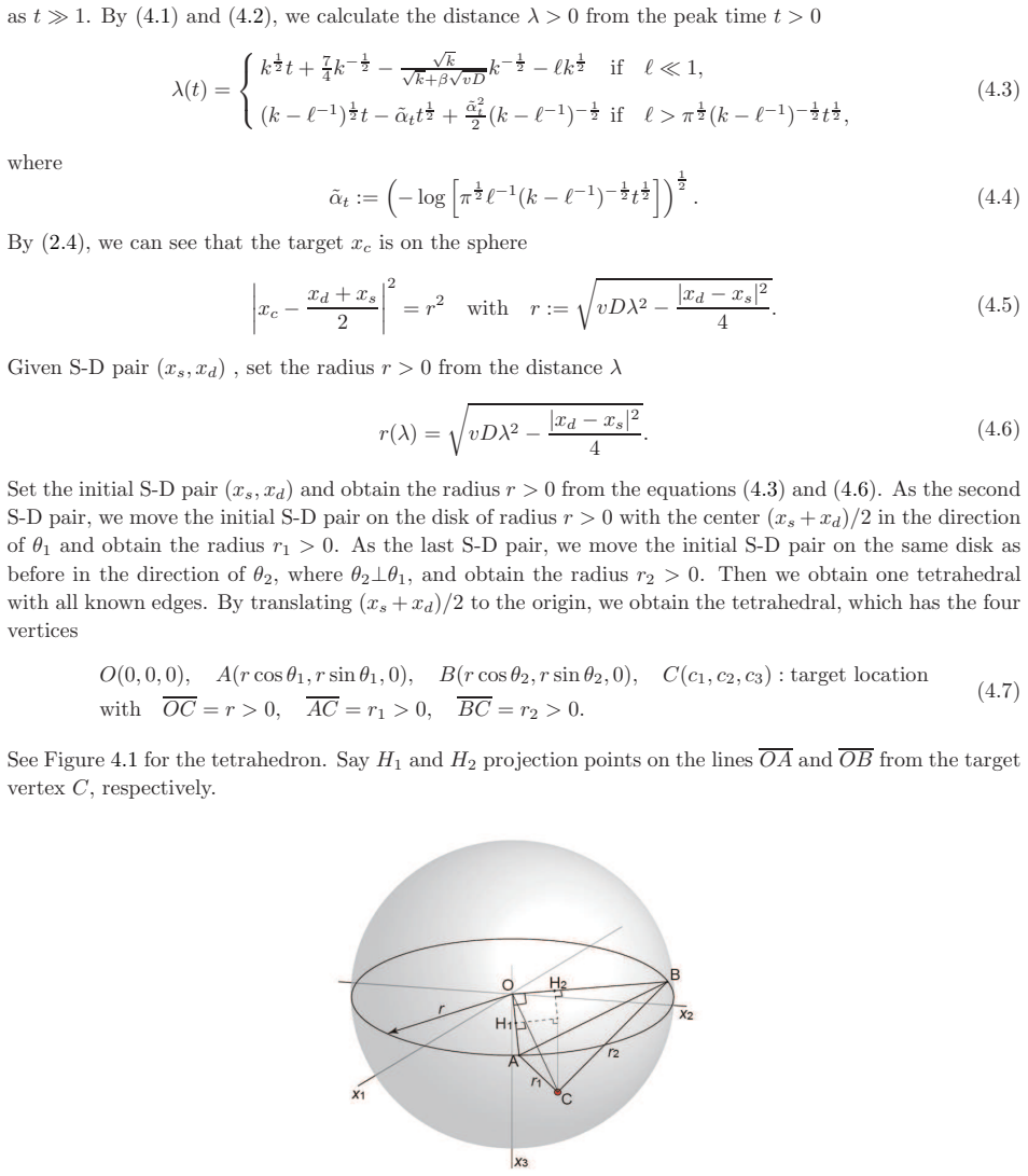
The central discovery is that the peak time of the emission signal can be inverted explicitly into the target-distance parameter $\lambda(t)$: for small fluorescence lifetime $\ell$, $\lambda(t) = k^{1/2}t + \frac{7}{4}k^{-1/2} - \frac{\sqrt{k}}{\sqrt{k}+\beta\sqrt{vD}}k^{-1/2} - \ell k^{1/2}$, and for large $\ell$, $\lambda(t) = (k-\ell^{-1})^{1/2}t - \tilde\alpha_t t^{1/2} + \frac{\tilde\alpha_t^2}{2}(k-\ell^{-1})^{-1/2}$, up to remainder terms. Once $\lambda$ is known, the identity $\lambda^2 = (|x_d-x_c|^2 + |x_s-x_c|^2)/(2vD)$ places the unknown target $x_c$ on the sphere centered at $(x_d+x_s)/2$ with radius $r = \sqrt{vD\lambda^2 - |x_d-x_s|^2/4}$. Three source-detector pairs give three such radii, which form the edges of a tetrahedron, and formulas (4.10) recover the target as the fourth vertex. In noise-free numerical tests the reconstruction errors are about 1.4% to 5.3% relative error for targets at depth 20-30 mm, and the depth estimate remains acceptable at 5% time-jitter noise.

Load-bearing premise

The argument assumes the measured peak time is close enough to the peak of the asymptotic profile $u^a_m$ that the expansions in (2.9) and (2.25), and their inversions in (4.3), apply; this closeness is checked numerically in Section 3 for selected parameters, but it is not proved for all source-detector-target configurations.

Editorial extensions

If this is right

Only three source-detector pairs are needed to recover a point target, and no iterative PDE solves or initial guesses are required.
The reconstruction is fully explicit: formulas (4.10) give the target coordinates directly from the three radii and two rotation angles.
The asymptotic analysis supplies error orders $O(t^{-1})$ for small lifetime and $O(t^{-1/2})$ for large lifetime, which the numerical experiments reflect as 1-5% relative error without noise.
Deeper targets at 30 mm depth reconstruct at least as accurately as shallower targets at 20 mm in the tests, consistent with the large-distance assumption $\lambda \gg 1$.
Time-jitter noise of 5% degrades the in-plane accuracy but still leaves a usable depth estimate, suggesting the method tolerates moderate measurement noise.
Because the work is a direct corollary of the paper's own claims, these consequences stand or fall with the asymptotic peak-time inversion.

Reading between the lines

Editorial extensions of the paper, not claims the author makes directly.

A natural testable extension would feed experimentally measured peak times from a tissue phantom into (4.3)-(4.10) and compare against known embedded fluorophore positions; the asymptotic error prediction says the error should shrink as source-detector-target distances grow.
Since the method needs only peak times rather than full temporal profiles, it might combine naturally with low-cost time-gated detectors; in practice the main experimental bottleneck is likely accurate calibration of the optical parameters $k$, $D$, $\mu_a$, $\beta$, and the lifetime $\ell$, since all enter $\lambda(t)$.
The tetrahedron construction suggests a geometric consistency check for redundant data: with more than three source-detector pairs, the reconstructed vertex should lie near the intersection of all the spheres, and disagreement among pairs could serve as a data-quality diagnostic.
If extended to non-point or multiple targets, the single-sphere argument likely breaks down unless the target distribution's peak-time signature is separated by lifetime or gating; the paper itself lists non-point targets and curved boundaries as future work.

Share X Bluesky LinkedIn Reddit HN

Signed reviews

No signed human review yet.

Editorial analysis

A structured set of objections, weighed in public.

Desk editor's note, referee report, and a circularity audit.

Desk Editor's Note

read the letter

What you should know: this is a genuine closed-form inversion for point-target time-domain FDOT in a homogeneous half-space. The asymptotic expansions in the small- and large-lifetime regimes are explicit, the numerics look encouraging, and the tetrahedron reconstruction is simple and clearly described. The main soft spot is that the paper does not bound the difference between the exact peak time and the approximate peak time used in the inversion.

What's new: Theorems 2.3 and 2.7 give asymptotic expansions for the approximate peak time, generalizing the authors' earlier equation (1.8) to (1.9) with a boundary-term correction. Equations (4.1)-(4.3) invert those expansions to produce a direct formula for the distance parameter lambda(t), and (4.5)-(4.10) turn three S-D pairs into the target location. I have not seen this explicit tetrahedron construction elsewhere. The derivations are internally consistent, and the paper is honest about the approximations.

Where it is soft: the stress-test point is the one that matters. The theorems control the approximate peak time, defined as the solution to (2.8) or (2.23), not the measured peak time of U_m. The gap between them is only verified numerically in Section 3 for a finite set of parameters. Since (4.3) has slope O(1) in t, a systematic offset delta-t shifts all three radii in (4.6) and the reconstructed vertex in (4.10). For large lifetimes the nominal remainder in (4.3) is only O(t^{-1/2}), which for t ~ 10^3 ps leaves errors of a few percent; the noise-free RelErr values in Tables 1 and 3 are consistent with that. The authors do not claim rigorous control, so this is a soft spot, not a fatal flaw. The noise experiments are single-sample per level, and no forward-solver code is shipped, so the figures cannot be independently reproduced. Those are addressable in revision.

Who this is for: anyone who wants a fast, non-iterative reconstruction of a single fluorescent point target in time-domain FDOT. It deserves refereeing because the core asymptotics are worked out carefully and the method is transparent. I would send it to a referee with a request to either prove a bound on the exact-approximate peak-time gap or demonstrate numerically that the gap stays small across a wider parameter range, and to add repeated noise runs. Engage with it; this is a serious paper that needs revision rather than rejection.

Referee Report

3 major / 5 minor

Summary. The paper proposes a direct, non-iterative inversion scheme for point-target fluorescence diffuse optical tomography (FDOT) using measured peak times of temporal response functions. The authors derive asymptotic expansions for an approximate peak time—defined as the critical point of an asymptotic profile of the emission solution—in two regimes: small fluorescence lifetime (Theorem 2.3) and large fluorescence lifetime (Theorem 2.7). These expansions are inverted to express the distance parameter λ in terms of peak time (Section 4, Eq. (4.3)), which determines a sphere on which the target lies (Eq. (4.5)). Using three source-detector pairs, the target is reconstructed as the vertex of a tetrahedron whose edges are the sphere radii (Eqs. (4.7)–(4.10)). Numerical experiments in Section 5 report noise-free reconstruction errors of roughly 1–5% and demonstrate robustness to time-jitter noise.

Significance. If the error between the approximate and the exact peak time could be rigorously controlled, this would be a valuable contribution: the scheme is explicit, avoids iterative optimization, uses peak-time measurements that are relatively robust to noise, and extends earlier peak-time formulas to include the extrapolation length β and nonzero fluorescence lifetime. The asymptotic formulas are closed-form and the tetrahedron reconstruction is straightforward to implement. The paper also provides numerical verification across several parameter sets. However, the central claim currently rests on an unproven link between the exact and approximate peak times and on a remainder estimate in the inversion that is not correct at the stated order, so the significance is conditional on those issues being resolved.

major comments (3)

[Section 2, Definitions 2.2/2.6 and Theorems 2.3/2.7; Section 4, Eq. (4.3)] The asymptotic theorems are stated for an approximate peak time defined as the critical point of the profile u_a^m, not for the exact peak time t_peak = argmax_t U_m used in the Inverse Problem of Section 1. Lemma 2.1 (Eq. (2.5)) gives only a pointwise approximation u_m = u_a^m(1+O(λ^{-1})), with no control of the derivative or of the argmax. Therefore applying the inversion (4.3) to a measured t_peak has no proven error bound. The numerical comparisons in Section 3, while supportive, are spot checks and do not supply the missing estimate. Since the entire inversion scheme is driven by measured peak times, this gap is load-bearing.
[Section 4, Eq. (4.2)] The replacement αλ = ᾶt + O(t^{-1/2}) is not correct at the stated order. From λ = (k−ℓ^{-1})^{1/2} t + O(t^{1/2}) one has λ^{1/2} = (k−ℓ^{-1})^{1/4} t^{1/2} + O(1), so αλ^2 = ᾶt^2 + O(t^{-1/2}) and hence αλ = ᾶt + O(t^{-1/2}/√log t). When the term −αλ t^{1/2} is expanded, the induced error in λ is O(t^{1/2} · t^{-1/2}/√log t) = O(1/√log t), not O(t^{-1/2}). Thus the final inversion formula (4.3) for ℓ ≫ 1 has a remainder that is only o(1), and its convergence is only logarithmic. At the finite times used in Section 5 (t ~ 10^2–10^3 ps), 1/√log t is of order 0.1–0.4, so the asymptotic analysis does not by itself explain the observed few-percent accuracy; the numerical success may rely on small constants not captured by the big-O estimates.
[Section 5, Eq. (4.10)] The algebraic reconstruction from the three radii r, r1, r2 is presented without any error propagation or conditioning analysis. The vertex formula (4.10) involves square roots and differences of fourth powers; small perturbations in the radii can be amplified, especially for nearly degenerate tetrahedra. The numerical tables cover only a few geometries and do not report the radii or the angles θ1, θ2, so the reader cannot assess the stability of the reconstruction. A quantitative sensitivity estimate is needed to support the claim that three peak-time measurements determine the target position accurately.

minor comments (5)

[Eqs. (1.5), (2.9), (4.1)] The notation in the β-dependent term is ambiguous; the denominator should be written consistently as √k + β√(vD), and the same expression should be used in (1.5), (2.9), and (4.1).
[Section 2, Lemma 2.5] Lemma 2.5 is quoted from the submitted manuscript [2] and its proof is not included. Please make the paper self-contained by providing a proof or a detailed proof sketch, especially because the lemma is the basis for the large-lifetime equation (2.23).
[Section 4, Eq. (4.4)] The definition of ᾶt requires the argument of the logarithm to lie in (0,1) for ᾶt to be real; this follows from the condition in (4.3) but should be stated explicitly.
[Section 5] Reporting the radii r, r1, r2 and the angles θ1, θ2 for the numerical examples would help the reader evaluate the conditioning of the tetrahedron reconstruction and reproduce the results.
[Throughout] There are several typographical and grammatical issues, e.g., 'unknwon' in Section 6, 'the proof the Theorem 2.7' at the end of the proof of Theorem 2.7, and redundant phrases such as 'is as in' in Section 3.

Circularity Check

0 steps flagged · score 0.0 of 10

No significant circularity; the inversion inverts a stated asymptotic model with physical parameters and is validated against the full PDE, not fitted to the target.

full rationale

The inversion chain is not circular. The paper defines an approximate peak time through explicit equations (2.8) and (2.23), derives asymptotic expansions t(lambda) in Theorems 2.3 and 2.7, and algebraically inverts those expansions to obtain lambda(t) in (4.3). No unknown target coordinate or strength is fitted to produce this relation; k, beta, v, D, and ell are stated physical parameters. The sphere relation (4.5)-(4.6) is an algebraic identity equivalent to the definition of lambda in (2.4), and the tetrahedron reconstruction (4.10) is exact geometry from the radii. The self-citations to [1] and [2] supply asymptotic lemmas, but those are prior mathematical results and are additionally checked in Section 3 against the full-PDE peak time, so the load-bearing relation is not merely an imported conclusion. The main gap is that the exact measured peak time is not proven to satisfy the approximate equations, only verified numerically; that is a validity and remainder-estimate concern, not a circular reduction of the output to the input.

Assumptions & free parameters 0 free parameters · 7 assumptions · 0 invented entities

The paper introduces no free parameters fitted to data; all constants are standard physical inputs. The main non-standard premises are the use of the authors' earlier asymptotic profile as a proxy for the exact solution, and the known-parameters assumption. These are stated or numerically supported, but not rigorously established. No new physical entities are postulated; the tetrahedron is a mathematical construction from measured radii, not an independent object with its own falsifiable predictions.

assumptions (7)

domain assumption Light transport in tissue is described by the coupled diffusion equations (1.1)-(1.2) with a Robin boundary condition.
Used as the forward model for excitation and emission; standard in FDOT, taken from [8]; the inversion inherits any modeling error.
domain assumption The fluorophore is a point target, mu(x) = c delta(x - x_c).
Inverse Problem in Section 1; all results are for a single point source; extension to extended targets is explicitly deferred to future work.
domain assumption The asymptotic profile u^a_m in (2.6) approximates u_m with relative error O(lambda^{-1}) under condition (2.3).
This is cited from the authors' prior work [1, Theorem 2.2 and Remark 2.3]; it is not re-proved here and it underpins the derivation of the peak-time equations.
ad hoc to paper The peak time of U_m can be replaced by the peak time of u^a_m, giving equations (2.8) and (2.23).
The only support is numerical comparison in Section 3; no rigorous error bound is given, and this substitution is what the inversion ultimately relies on.
domain assumption In Proposition 2.4, the relation x_c3 ~ sqrt(vD) lambda is used for the boundary correction.
Used to simplify the correction term in (2.15); it is a geometric scaling assertion for boundary source/detector pairs and target depth.
standard math The large-lifetime inversion uses the saddle-point estimate Lemma 2.5 and the conditions t > lambda (k - ell^{-1})^{-1/2} and condition (2.24).
The saddle-point estimate is standard analysis; the conditions delimit the regime where the approximate peak-time equation has a unique positive solution.
domain assumption Optical parameters v, D, mu_a, beta, and ell are known exactly.
The inversion formulas (4.3) require all these as inputs; no uncertainty or parameter recovery is treated.

how reviews work

0 comments

Cite this review

Pith. "Pith review of Direct inversion scheme of time-domain fluorescence diffuse optical tomography by asymptotic analysis of peak time." pith.science (2026). https://pith.science/paper/R7WMVAWX

@misc{pith2026250201037,
  author       = {Pith},
  title        = {Pith review of: Direct inversion scheme of time-domain fluorescence diffuse optical tomography by asymptotic analysis of peak time},
  year         = {2026},
  howpublished = {\url{https://pith.science/paper/R7WMVAWX}},
  note         = {Machine review of arXiv:2502.01037}
}

read the original abstract

This paper proposes a direct inversion scheme for fluorescence diffuse optical tomography (FDOT) to reconstruct the location of a point target using the measured peak time of the temporal response functions. A sphere is defined for the target, with its radius determined by the peak time, indicating that the target lies on the sphere. By constructing a tetrahedron with edges determined by the radii, we identify the location of the target as the vertex of the tetrahedron. Asymptotically, we derive the relationship between the radius of the sphere and the peak time. Several numerical tests are implemented to demonstrate the accuracy and performance of the asymptotic relationship and the inversion scheme.

Figures

Figures reproduced from arXiv: 2502.01037 by the authors.

**Figure 3.1.** Peak time tpeak and the asymptotic t s peak. For (b) and (c), we set ℓ = 100 ps. In [PITH_FULL_IMAGE:figures/full_fig_p009_3_1.png] view at source ↗

**Figure 3.2.** Peak time tpeak and the approximate peak time t l0 peak. For (b) and (c), we set ℓ = 1000 ps. (a) (b) (c) 500 1000 1500 2000 400 500 600 700 800 900 1000 1100 0.05 0.1 0.15 0.2 200 400 600 800 1000 1200 1400 10 15 20 25 30 35 40 600 800 1000 1200 1400 1600 1800 2000 2200 [PITH_FULL_IMAGE:figures/full_fig_p010_3_2.png] view at source ↗

**Figure 3.3.** Peak time tpeak and the approximate peak time t l peak. For (b) and (c), we set ℓ = 1000 ps. λ > 0. When ℓ ≪ 1, by (2.9), one can easily obtain λ = k 1 2 t + 7 4 k − 1 2 − √ k √ k + β √ vD k − 1 2 − ℓk 1 2 + O [PITH_FULL_IMAGE:figures/full_fig_p010_3_3.png] view at source ↗

Figures from the paper (1 more)

**Figure 4.1.** Figure 4.1: Tetrahedron with four vertices O, A, B and C. Point A is the center point of the initial S-D pair. Points B and C are the center points of the second and third S-D pairs, respectively. Point C is the target location. Write the x, y-coordinates of the vertex C as c1 =…

Discussion (0). Continue with ORCID to comment.

Reference graph

Works this paper leans on

11 extracted references · 11 canonical work pages

[1]

S. Chen, J. Eom, G. Nakamura, G. Nishimura, Approximate peak t ime and its application to time- domain ﬂuorescence diﬀuse optical tomography, Commun. Anal. Comput. , 1 (2023) 379–406

work page 2023
[2]

S. Chen, J. Eom, G. Nakamura, G. Nishimura, Approximate peak t ime to time-domain ﬂuorescence diﬀuse optical tomography for nonzero ﬂuorescence lifetime, sub mitted

work page
[3]

J. Eom, M. Machida, G. Nakamura, G. Nishimura, C. Sun, Express ions of the peak time for time-domain boundary measurements of diﬀuse light, J. Math. Phys. , 64 (2023) 083504

work page 2023
[4]

J. Eom, G. Nakamura, G. Nishimura, C. Sun, Local analysis for loc ating a single point target in time- domain ﬂuorescence diﬀuse optical tomography, Diﬀer. Integral Equ. 37 (2024) 27–58

work page 2024
[5]

Hebden, R

J. Hebden, R. Kruger, K. Wong, Time resolved imaging through a h ighly scattering medium, Appl. Opt., 30 (1991) 788–794

work page 1991
[6]

Jiang, Diﬀuse optical tomography: principles and applications , CRC Press, Boca Raton, 2010

H. Jiang, Diﬀuse optical tomography: principles and applications , CRC Press, Boca Raton, 2010. 14

work page 2010
[7]

Jiang, Fluorescence Molecular Tomography: Principles and Applic ations, Springer, Cham, Switzer- land, 2022

H. Jiang, Fluorescence Molecular Tomography: Principles and Applic ations, Springer, Cham, Switzer- land, 2022

work page 2022
[8]

J. Liu, M. Machida, G. Nakamura, G. Nishimura, C. Sun, On ﬂuores cence imaging: the diﬀusion equation model and recovery of the absorption coeﬃcient of ﬂuorophores , Sci. China Math. , 65 (2022) 1179–1198

work page 2022

Show all 11 references

[9]

Y. Liu, W. Ren, H. Ammari, Robust reconstruction of ﬂuorescen ce molecular tomography with an optimized illumination pattern, Inverse Probl. Imag. 14 (2020) 535–568

2020
[10]

Mycek, B

M. Mycek, B. Pogue, Handbook of Biomedical Fluorescence , Marcel Dekker, New York, 2003

2003
[11]

Nitziachristos, C

V. Nitziachristos, C. Tung, C. Bremer, R. Weissleder, Fluoresc ence molecular tomography resolves protease activity in vivo, Nat. Med., 8 (2002) 757–761. 15

2002

Pith tools

Reviewed August 9, 2026 · model on record in the stance chip above.

[1] [1]

S. Chen, J. Eom, G. Nakamura, G. Nishimura, Approximate peak t ime and its application to time- domain ﬂuorescence diﬀuse optical tomography, Commun. Anal. Comput. , 1 (2023) 379–406

work page 2023

[2] [2]

S. Chen, J. Eom, G. Nakamura, G. Nishimura, Approximate peak t ime to time-domain ﬂuorescence diﬀuse optical tomography for nonzero ﬂuorescence lifetime, sub mitted

work page

[3] [3]

J. Eom, M. Machida, G. Nakamura, G. Nishimura, C. Sun, Express ions of the peak time for time-domain boundary measurements of diﬀuse light, J. Math. Phys. , 64 (2023) 083504

work page 2023

[4] [4]

J. Eom, G. Nakamura, G. Nishimura, C. Sun, Local analysis for loc ating a single point target in time- domain ﬂuorescence diﬀuse optical tomography, Diﬀer. Integral Equ. 37 (2024) 27–58

work page 2024

[5] [5]

Hebden, R

J. Hebden, R. Kruger, K. Wong, Time resolved imaging through a h ighly scattering medium, Appl. Opt., 30 (1991) 788–794

work page 1991

[6] [6]

Jiang, Diﬀuse optical tomography: principles and applications , CRC Press, Boca Raton, 2010

H. Jiang, Diﬀuse optical tomography: principles and applications , CRC Press, Boca Raton, 2010. 14

work page 2010

[7] [7]

Jiang, Fluorescence Molecular Tomography: Principles and Applic ations, Springer, Cham, Switzer- land, 2022

H. Jiang, Fluorescence Molecular Tomography: Principles and Applic ations, Springer, Cham, Switzer- land, 2022

work page 2022

[8] [8]

J. Liu, M. Machida, G. Nakamura, G. Nishimura, C. Sun, On ﬂuores cence imaging: the diﬀusion equation model and recovery of the absorption coeﬃcient of ﬂuorophores , Sci. China Math. , 65 (2022) 1179–1198

work page 2022