Impact of Hill coefficient and time delay on a perceptual decision-making model

Anna Czartoszewska; Bart{\l}omiej Morawski

REVIEW 4 major objections 5 minor 15 references

Impact of Hill coefficient and time delay on a perceptual decision-making model

T0 review · 4 major / 5 minor · reviewed 2026-08-07 · deepseek-v4-flash

Challenge this review Re-run · record.json Download PDF Read on arXiv ↗

Pith's one-line read Treating synapse weights as a separate dynamic variable can reverse the predicted fate of a delayed perceptual decision network.

desk verdict Clean analytical generalization of a known decision-making model, but the showcase divergence between the two- and three-equation systems is demonstrated exactly where the quasi-steady-state reduction is least trustworthy. read the letter →

arxiv 2506.19853 v1 pith:REUCDUTH submitted 2025-06-04 q-bio.NC math.DS

Bart{l}omiej Morawski , Anna Czartoszewska This is my paper · ORCID

classification q-bio.NCmath.DS MSC 34K6034C6092B0592C20

keywords perceptualdecisionmakingHillfunctiondelaydifferentialequationssynapticfacilitationwinner-take-allHopfbifurcationquasi-steadystateapproximationneuralmassmodel

verification ladder T0 review T1 audit T2 compute T3 formal

The pith

A machine-rendered reading of the paper's core claim, the machinery that carries it, and where it could break.

The reading

The paper is trying to establish that the perceptual decision-making model of Piskała et al. -- two neural populations competing through plastic synapses with delayed self-inhibition -- behaves differently depending on two generalization choices: the Hill coefficient $n$ of the facilitation function and whether the synaptic weights are kept as dynamic variables or frozen at their quasi-steady state. For symmetric inputs, the number of steady states is controlled by the function $I = g_n(r)=r-\epsilon r f_n(r^2)$, with $\epsilon = 8n/(2n+1)^2$ as the threshold separating a unique equilibrium from bistable regimes. The authors derive closed-form critical delays $\tau_0^1,\tau_0^2$ at which each reduced model loses stability through a Hopf bifurcation, and show numerically that for one parameter set the two reductions disagree qualitatively: the two-equation quasi-steady-state version oscillates with growing amplitude and produces a negative firing rate near $t=28$, while the three-equation equal-weight version converges to a steady state. If the paper is right, the choice of approximation is not innocuous: models that look equivalent near equilibrium can give opposite answers in the parameter regimes that matter for real decisions.

What carries the argument

The machinery has three pieces. The Hill function $f_n(r_1r_2)=(r_1r_2)^n/(1+(r_1r_2)^n)$ encodes short-term synaptic facilitation, entering both the weight dynamics and, through $g_n(r)=r-\epsilon r f_n(r^2)$, the steady-state condition $I=g_n(r)$. For delay stability, the characteristic determinant is factored into exponentials of the form $a\lambda+b+e^{-\lambda\tau}$ (two-equation model) or $a\lambda^2+b\lambda+c+(\alpha\lambda+\beta)e^{-\lambda\tau}$ (three-equation model); a standard transcendental-root theorem fixes the imaginary-axis crossing and gives the closed-form critical delays, and a Hopf theorem turns the crossing into a periodic solution. The quasi-steady-state system is System (5), the equal-weight system is System (13), and their comparison is the paper's main numerical object.

What would settle it

Integrate the full four-equation System (1) numerically for coefficient set 3 with matched initial conditions $w_1(0)=w_2(0)=\epsilon f_n(r_1^0 r_2^0)$ and compare with Figures 9(a) and 9(b): if the full system stays positive and converges to the steady state, the quasi-steady-state reduction is wrong in that regime; if it develops growing oscillations and a negative firing rate near $t=28$, the equal-weight reduction is the misleading one.

Watch

Extended reading notes

Core claim

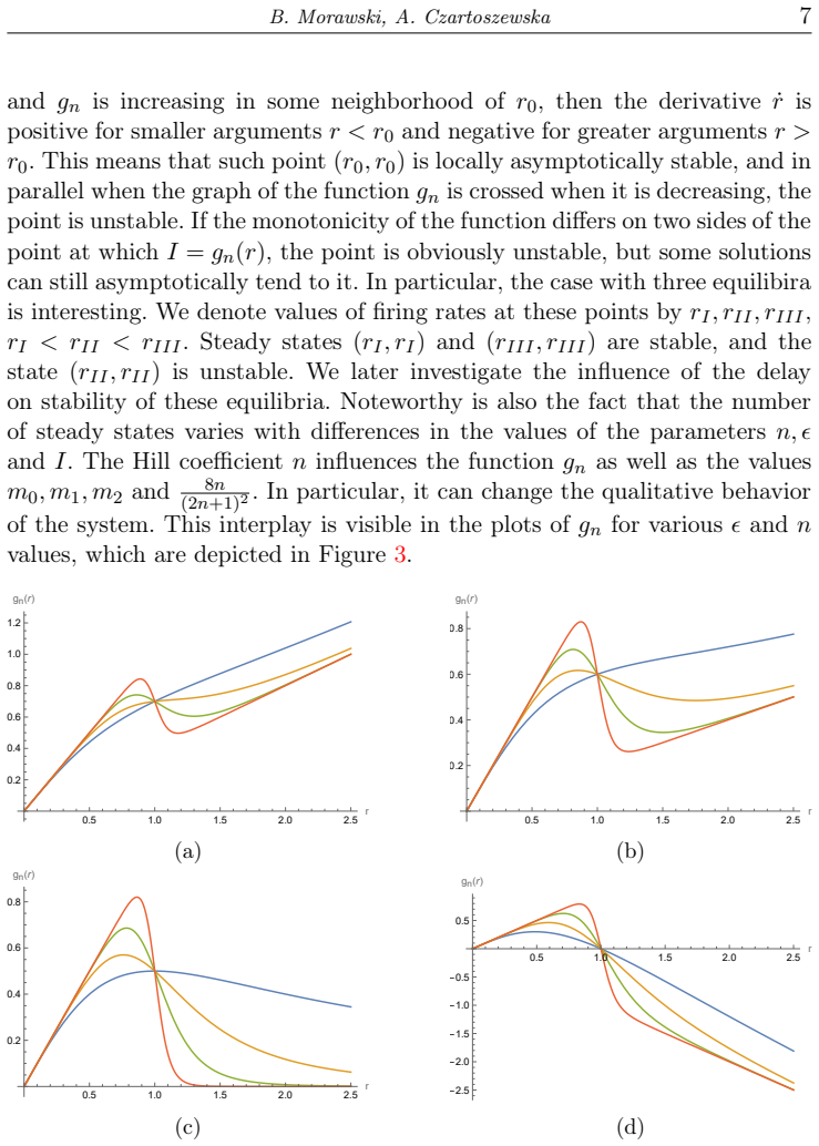
The central claim is that the extension of the Piskała--Bielczyk--Foryś model to arbitrary $n\ge 1$ and to a three-equation equal-weight variant preserves the steady-state and Hopf-bifurcation framework of the earlier $n=2$ analysis, but introduces a genuine discrepancy between the two reductions. The function $g_n$ determines the equilibria and their stability in the symmetric case $I_1=I_2$, and the threshold $\epsilon = 8n/(2n+1)^2$ marks where the system can switch from one to three steady states. Linearizing the delayed systems factorizes the characteristic equation into factors of the form $a\lambda+b+e^{-\lambda\tau}$, allowing the authors to write the critical delays in closed form; in the two-equation System (5) the smaller delay always lies in $(\tau_r,\tau_r\pi/2)$, whereas in the three-equation System (13) the ordering of the two critical delays depends on $\tau_w$ and can reverse. The numerical comparison then shows that, for $n=2$, $\epsilon=0.6$, $\tau=1.2$, $I_1=0.6$, $I_2=0.7$, $\tau_r=1$, $\tau_w=0.5$, System (13) appears to settle to a steady state while System (5) oscillates with increasing amplitude and a firing rate becomes negative around $t=28$, indicating that the quasi-steady-state approximation and the equal-weight assumption are not interchangeable in this regime.

Load-bearing premise

The load-bearing premise is that a neuron population's synaptic weight can be treated as instantaneously at its equilibrium value whenever the firing rates move slowly; the paper's own discussion says no rigorous justification for this approximation is supplied, and if it fails the two-equation model's predictions would not describe the original four-equation system.

Editorial extensions

If this is right

For symmetric inputs, increasing the Hill coefficient $n$ lowers the bistability threshold $\epsilon = 8n/(2n+1)^2$, so neurons with steeper facilitation curves need a smaller maximal synaptic weight before a second and third steady state can appear.
In the two-equation model, the stable steady state always loses stability through a Hopf bifurcation at a delay in $(\tau_r,\tau_r\pi/2)$, because $\tau_0^1<\tau_0^2$ always; in the three-equation model this ordering can reverse, so the identity of the destabilizing mode depends on the plasticity time scale $\tau_w$.
A steady state that is unstable with no delay cannot be stabilized by increasing the delay, in either reduced model.
The numerical example with $\tau=1.2$, $n=2$, $\epsilon=0.6$ shows that the two reductions predict opposite qualitative behavior at the same parameters, so conclusions drawn from the quasi-steady-state model near the instability threshold should be checked against the equal-weight model.

Reading between the lines

Editorial extensions of the paper, not claims the author makes directly.

Editorial inference: the full four-equation system provides a natural referee for the discrepancy; computing its solution for coefficient set 3 would decide which reduced model is faithful there, and the paper leaves this computation for the future.
Editorial inference: because the divergence in System (5) coincides with a firing rate crossing zero, a likely observable signature of the quasi-steady-state approximation's failure is the appearance of biologically impossible negative rates; monitoring positivity of the reduced models is therefore a cheap validity check.
Editorial inference: the paper's transient overshoot, where $r_1>r_2$ although $r_2$ has larger input and initial condition, implies that any decision rule based on a snapshot of firing rates is unreliable; extending the model with explicit decision times and error rates would turn this observation into a testable prediction.

Share X Bluesky LinkedIn Reddit HN

Editorial analysis

A structured set of objections, weighed in public.

Desk editor's note, referee report, and a circularity audit.

Desk Editor's Note

read the letter

Quick take: this is a legitimate, mostly clean extension of the Piskała–Bielczyk–Foryś line of work. The genuinely new pieces are the three-equation equal-weight model and the generic-Hill-coefficient analysis. I checked the two key symbolic steps — the bistability threshold 8n/(2n+1)^2 from the function g_n and the factorization of the 3x3 characteristic determinant — and both are fine. The critical-delay formulas (16) and (25) follow from the stated Cooke–van der Driessche theorem, and the paper is careful about when the Hopf argument applies, including the remark about integer multiples of the crossing frequencies. The steady-state and stability picture in Section 2.1, read off the shape of g_n, is clear, honest, and geometrically satisfying.

Where I get off the train is the headline claim: System (13) converging while System (5) diverges rests on a single finite-time simulation with asymmetric inputs (Fig. 9, coefficient set 3). The stress-test point lands. Every simulation runs at tau_w/tau_r = 0.5, the quasi-steady-state reduction is motivated by tau_w much smaller than tau_r, and the authors explicitly concede they lack a rigorous justification for the approximation. So the comparison is made exactly where the two-equation model is least reliable, and the analytic stability results do not cover the asymmetric inputs used in that figure. The growing oscillations — and the firing rate going negative near t = 28 — may well be an artifact of the approximation rather than a genuine modeling consequence. That does not undermine the analytic core, but it means the paper's most visible result is a conjecture supported by one simulation, not an established fact.

Lesser issues: the statement that System (13) appears to converge wants a longer time horizon or, better, a robustness check across initial conditions and nearby parameters; the placeholder DOI and the received/revised dates (2017 on a 2025 submission) are mechanical and should be cleaned up. The citation practice is appropriate — the debt to Foryś et al. and Bielczyk et al. is disclosed, and the new results are genuinely new relative to them.

Bottom line: this paper is for people working on this specific model family and for anyone worried about reduction artifacts in neural-mass models. The math deserves a serious referee even though the headline needs to be reined in. I would send it to peer review and ask the authors to either justify the quasi-steady-state reduction at their parameter values — via perturbation theory, as they themselves suggest, or by direct numerical comparison against the full four-equation System (1) — or soften the claim accordingly.

Referee Report

4 major / 5 minor

Summary. The paper analyzes a neural-mass model of perceptual decision making that includes two populations with plastic synaptic weights and delayed self-inhibition. It generalizes earlier work by allowing a generic Hill coefficient n≥1 and by introducing a three-equation variant in which the two synaptic weights are assumed equal. The authors derive steady-state conditions and critical delay values for Hopf bifurcation in the symmetric-input case, and they numerically compare the two-equation quasi-steady-state model with the three-equation model. For one parameter set they report a qualitative difference: the three-equation system appears to converge while the two-equation system exhibits growing oscillations that eventually make a firing rate negative.

Significance. The analytical parts of the paper are a genuine and mostly correct generalization of the earlier n=2 results: the threshold 8n/(2n+1)^2 for bistability, the factorization of the characteristic determinants, and the critical-delay formulas for symmetric inputs are derived carefully and are useful for the mathematical neuroscience community. The three-equation model is a natural intermediate between the full four-equation model and the quasi-steady-state two-equation model, and the observation that different modeling choices can affect qualitative predictions is potentially valuable. However, the central numerical claim rests on a quasi-steady-state approximation in a parameter regime where that approximation is not justified, and the paper explicitly concedes the lack of a rigorous justification. The paper also ships no code or numerical details, so the headline comparison is not independently reproducible as reported. If the approximation issue is repaired and the comparison is validated against the full model, the paper would make a solid contribution; in its current form the main claim is not established.

major comments (4)

[§2.1, Eq. (3)] The statement that "Solutions to System (3) are also solutions to System (2)" is not correct. If (r1,r2) solves System (3) and one defines w1=w2=ϵf(r1r2), then the right-hand sides of the w-equations in System (2) vanish, but the time derivative of ϵf(r1r2) is generally nonzero along the solution. Hence System (3) is a quasi-steady-state approximation rather than an exact reduction, as the Discussion (p. 27) implicitly concedes. This invalidates the accompanying global-existence argument and leaves the validity of the two-equation model (5) unestablished. The authors should either prove an approximation estimate (for example via Tikhonov's theorem, which they mention on p. 27) or validate System (5) against the full four-equation system numerically for the parameter sets actually used.
[§3, Table 1 and Fig. 9] The headline qualitative difference between Systems (13) and (5) is exhibited for coefficient set 3, where τw/τr = 0.5/1 = 0.5. Section 2.1 motivates the quasi-steady-state reduction by assuming that τw is "much smaller" than τr, so the comparison is made exactly in a regime where the reduction underlying System (5) is not justified. Since System (5) is the approximate model, the growing oscillations and the negative firing rate around t=28 in Fig. 9(b) may be artifacts of the approximation rather than a genuine consequence of treating w as a separate variable. The numerical comparison should be repeated for τw/τr ≪ 1 and/or validated against the full four-equation System (1).
[§2.1, symmetric-input paragraph] The claim that "All solutions of the System (3) with symmetric inputs lay on the straight line r1=r2=r" is false: for r1(0)≠r2(0) the difference obeys u'= -u(1+ϵf(r1r2))/τr and decays exponentially but is not identically zero for positive time. The subsequent stability conclusion is nevertheless correct because the transverse direction is contracting, but the proof should be restated in terms of this contraction rather than asserting that all solutions lie on the diagonal.
[§2.2–2.3 vs §3] The analytical critical-delay results (Eqs. (11), (16), (25)) are derived under the assumption of symmetric inputs I1=I2, yet the numerical demonstration of the qualitative difference in Fig. 9 uses asymmetric inputs I1=0.6, I2=0.7. Consequently the headline result is not connected to the analytical stability and bifurcation analysis and rests entirely on the numerical simulations identified in the previous comment. The authors should either extend the analysis to asymmetric inputs or clearly restrict the claim and provide a supporting symmetric-input example.

minor comments (5)

[Fig. 7(f) and surrounding text] The text refers to the "non-monotonicity of the weight w" in Fig. 7(f), but System (5) has no dynamic weight variable; the plot shows the time-dependent steady-state value ϵf(r1r2). Please rephrase to avoid confusion.
[§3, numerical methods] The numerical section gives no solver tolerances, step sizes, or code; adding these details would improve reproducibility.
[§2.3, sign of sin(y+τ)] The sign condition for sin(y+τ) is stated to hold under τw≤τr, but this inequality is not guaranteed for the general model; please state explicitly where this assumption is used and whether the main claims depend on it.
[Title page] There are numerous spacing errors in the author names and affiliations (e.g., "Bar tłomiej Mora wski", "W arsa w") that should be corrected in the final version.
[Theorem 2.1] The phrasing "if z is a simple root and s≠0, then y is a simple root of F(y)=0" appears to reverse the logical order of the theorem; the intended statement is that a simple real root of F corresponds to a simple root crossing the imaginary axis.

Circularity Check

0 steps flagged · score 0.0 of 10

No significant circularity: the analytical results are derived from the model equations by calculus and linearization, with no fitted parameters and no load-bearing self-citations.

full rationale

The paper's derivation chain is self-contained. The bistability threshold 8n/(2n+1)^2 follows directly from differentiation of the function g_n in Eq. (4), and the critical delay formulas in Eqs. (11), (16), and (25) are obtained by applying the standard Cooke–van der Driessche theorem and Hopf bifurcation theory to the characteristic equations of Systems (5) and (13). No parameter is fitted to data, and no 'prediction' is a renamed input. The cited prior work [5] and [6] provides the baseline n=2 model, but the paper re-derives and generalizes the analysis to n>=1 and to the three-equation system, so the citations are not load-bearing for the new claims. The numerical simulations merely illustrate the analytical and model-comparison results. The Discussion's explicit caveat that the quasi-steady-state approximation lacks rigorous theoretical justification is a validity and correctness limitation of the modeling reduction, not a circularity: it does not mean that any output is equivalent by construction to an input. Accordingly, no circular step can be exhibited, and the appropriate circularity score is 0.

Assumptions & free parameters 6 free parameters · 7 assumptions · 0 invented entities

The central derivations rest on standard DDE stability theory and on modeling assumptions inherited from the original model. No new physical entities are introduced; the three-equation model is an exact reduction on the invariant manifold w1=w2, not a new postulated mechanism. The quasi-steady-state approximation is the least-supported axiom and is acknowledged as such by the authors.

free parameters (6)

Hill coefficient n
Model parameter scanned in numerics (n=1,2,4); not fitted to data. Analytical results hold for general n>=1.
Maximal synapse strength epsilon
Scanned values 0.2-0.8 in Figures 5-6 and 0.6/0.72 in Table 1; not fitted.
Self-inhibition delay tau
Scanned values 0.6, 0.8, 0.9, 1.2 in Table 1 and Figures 5-6; not fitted.
Inputs I1, I2
Constant inputs; set to 0.6 and 0.7 in numerics; analytic results assume I1=I2=I.
Time scales tau_r, tau_w
Set to tau_r=1 and tau_w=0.3/0.5/0.8 in numerics; tau_r scales the delay formulas.
Initial firing rates r0_1, r0_2
Chosen per parameter set (e.g., 0 and 1); initial weights set to steady-state value, equal to 0 for the chosen sets.

assumptions (7)

standard math Cooke-van der Driessche theorem (Theorem 2.1) characterizes imaginary-axis crossings of characteristic roots for P(z)+Q(z)e^{-tau z}=0.
Used in Sections 2.2 and 2.3 to locate the first critical delay at which stability is lost.
standard math Hopf bifurcation theorem (Theorem 2.2) guarantees periodic solutions when a simple imaginary root crosses the imaginary axis with non-zero speed and no resonances.
Invoked in Sections 2.2 and 2.3 to conclude that a Hopf bifurcation occurs at tau=tau0.
domain assumption Inputs I1 and I2 are constant in time, making the systems autonomous.
Stated in Section 1.2 and used throughout; the authors acknowledge this limits generalizability.
domain assumption The quasi-steady-state approximation w_i = epsilon f(r1 r2) is valid for short-term plasticity.
Used to derive Systems (3) and (5); the authors admit there is no rigorous justification (Discussion, p. 27).
domain assumption The Hill function f_n(r1 r2) = (r1 r2)^n / (1 + (r1 r2)^n) with n>=1, and n>1 produces no significant qualitative changes in f_n's shape.
Section 1.2; the paper then analyzes n-dependent effects, so the 'no significant changes' claim is informal.
domain assumption Symbolic stability analysis is restricted to symmetric inputs I1=I2, so steady states satisfy r1=r2.
Sections 2.2-2.3 assume this to factorize the characteristic equation; numerical simulations use asymmetric inputs.
domain assumption The inequality tau_w <= tau_r is assumed to determine the sign of sin(y+ tau) for the critical delay in the three-equation model.
Section 2.3, Eq. (23) discussion; the numerical parameter sets satisfy this.

how reviews work

0 comments

Cite this review

Pith. "Pith review of Impact of Hill coefficient and time delay on a perceptual decision-making model." pith.science (2026). https://pith.science/paper/REUCDUTH

@misc{pith2026250619853,
  author       = {Pith},
  title        = {Pith review of: Impact of Hill coefficient and time delay on a perceptual decision-making model},
  year         = {2026},
  howpublished = {\url{https://pith.science/paper/REUCDUTH}},
  note         = {Machine review of arXiv:2506.19853}
}

read the original abstract

In this paper, a neural mass perceptual decision making model introduced by Piska{\l}a et al. is analyzed. The model describes activity of two neuron populations influenced by each other and external inputs. The groups' activities correspond to the process of making a perceptual binary decision. Existing results are generalized by investigating the impact of both a delay in self-inhibition and a generic Hill coefficient on solutions to the system of differential equations. Several versions of the model with various assumptions are compared using analytical and numerical methods.

Figures

Figures reproduced from arXiv: 2506.19853 by the authors.

**Figure 1.** Scheme of the modeled system. In the analyzed model, synaptic plasticity of the connections between the populations is incorporated using differential equations describing changes in connection weights, denoted by w1(t) and w2(t). Their magnitudes are influenced by the activity of the populations, and the maximum strength of a synaptic connection is anatomically limited, with the maximum denoted by ϵ. We assume that… view at source ↗

**Figure 2.** Shape of the Hill function fn depending on the parameter n [PITH_FULL_IMAGE:figures/full_fig_p003_2.png] view at source ↗

**Figure 3.** The plot of the function gn for n = 1, 2, 4, 10 in blue, yellow, green and red, respectively with (a) ϵ = 0.6, (b) ϵ = 0.8, (c) ϵ = 1 and (d) ϵ = 2. The parameter n has clear influence on shape of the function gn, and therefore on qualitative behavior of solutions for certain inputs [PITH_FULL_IMAGE:figures/full_fig_p007_3.png] view at source ↗

Figures from the paper (10 more)

**Figure 4.** Figure 4: The plot of the function g(x) = arccos √ x 1−x2 , where limx→−1 g(x) = ∞ and limx→1 g(x) = 1. Assuming other parameters to be constant, the delay τ 1 0 is decreasing with respect to ϵ, while τ 2 0 is increasing. This follows from the monotonicity of the function g and …

**Figure 5.** Figure 5: The plot of τ0 as a function of n for ϵ = 0.2, 0.4, 0.6, 0.8 in blue, yellow, green and red, respectively with (a) r = 0.3, (b) r = 0.5, (c) r = 0.7 and (d) r = 2. By choosing the value of r, the corresponding input I is determined and there exist inputs for which each…

**Figure 6.** Figure 6: The plots of τ 2 0 (solid lines) and τ 1 0 (dotted lines) as functions of n for ϵ = 0.2, 0.4, 0.6, 0.8 in blue, yellow, green and red, respectively with (a) τw = 0.3, r = 0.7, (b) τw = 0.8, r = 0.7, (c) τw = 0.3, r = 2 and (d) τw = 0.8, r = 2. By choosing the value of …

**Figure 7.** Figure 7: The plots for the coefficient set 1 from [PITH_FULL_IMAGE:figures/full_fig_p019_7.png]

**Figure 8.** Figure 8: The plots for the coefficient set 2 from [PITH_FULL_IMAGE:figures/full_fig_p020_8.png]

**Figure 9.** Figure 9: The plots for the coefficient set 3 from [PITH_FULL_IMAGE:figures/full_fig_p021_9.png]

**Figure 10.** Figure 10: The plots for the coefficient set 4 from [PITH_FULL_IMAGE:figures/full_fig_p022_10.png]

**Figure 11.** Figure 11: The plots for the coefficient set 5 from [PITH_FULL_IMAGE:figures/full_fig_p023_11.png]

**Figure 12.** Figure 12: The plots for the coefficient set 6 from [PITH_FULL_IMAGE:figures/full_fig_p024_12.png]

**Figure 13.** Figure 13: The plots for the coefficient set 7 from [PITH_FULL_IMAGE:figures/full_fig_p025_13.png]

Discussion (0). Continue with ORCID to comment.

Reference graph

Works this paper leans on

15 extracted references · 15 canonical work pages

[1]

Impact of Hill coefficient and time delay on a perceptual decision-making model

Introduction 1.1. Neuroscientific context Decision making is one of the most important functions of the brain, enabling humans and other animals to function in everyday life. Apart from complex, conscious decisions, our brain makes many perceptual decisions that we may not be aware of, concerning observed shapes, colors, direction of movement, location of...

work page Pith review arXiv 2025
[2]

The first one is a quasi-steady state approximation, which reduces the original four equations to two equations for firing ratesr 1,2

Model analysis In this chapter, we investigate two simplified versions of System (1). The first one is a quasi-steady state approximation, which reduces the original four equations to two equations for firing ratesr 1,2. The other one allows the weights to not be in their steady state, but assumes them to be equal, resulting in a three-equation system. No...

work page
[3]

Let alsoF:R→Rbe a real function defined asF(y) =|P(iy)| 2−|Q(iy)|2 and s= sgnF ′(y)denote the sign of its derivative

P(iy) =P( iy), Q(iy) =Q( iy)fory∈R, 3.P(0) +Q(0)̸= 0. Let alsoF:R→Rbe a real function defined asF(y) =|P(iy)| 2−|Q(iy)|2 and s= sgnF ′(y)denote the sign of its derivative. Then for variablesτ, z=iy, y∈R + satisfying the equation P(z) +Q(z)e −τ z= 0(8) the following holds: ifzis a simple root ands̸= 0, thenyis a simple root of F(y) = 0and the rootz(τ)of Eq...

work page
[4]

-1.0 -0.5 0.0 0.5 1.0 x 1 2 3 4 5 6 g(x) Figure 4: The plot of the functiong(x) =arccosx√ 1−x2, wherelim x→−1 g(x) =∞ andlim x→1 g(x) = 1

Moreover,g(0) = π 2, limx→1 g(x) = 1and ϵ·(f(r 2) + 2r2f ′(r2)) >0, which impliesτ 1 0 ∈(τ r, τrπ 2 ) regardless of the values ofr,ϵandn. -1.0 -0.5 0.0 0.5 1.0 x 1 2 3 4 5 6 g(x) Figure 4: The plot of the functiong(x) =arccosx√ 1−x2, wherelim x→−1 g(x) =∞ andlim x→1 g(x) = 1. Assuming other parameters to be constant, the delayτ1 0 is decreasing with respe...

work page
[5]

The simulations were performed using Wolfram Mathematica 13.0 and the built-in delay differential equation solving tools

Numerical simulations In this section Systems (5) and (13) are investigated using numerical methods. The simulations were performed using Wolfram Mathematica 13.0 and the built-in delay differential equation solving tools. We compare the behavior of solutions of the two systems for different sets of nine coefficients: •ϵ, τ, n– the maximal synapse capacit...

work page
[6]

[6] and then extended by Foryś et al

Discussion In this work, we introduced and analyzed a few variants of the model first proposed by Piskała et al. [6] and then extended by Foryś et al. [5] and Bielczyk et al. [1]. We considered basic properties of the full four-equation model describing the firing rates of two neural populations and the weights of their synaptic connections. Then we analy...

work page
[7]

N. Z. Bielczyk, K. Piskała, M. Płomecka, P. Radziński, L. Todorova, and U. Foryś. Time-delay model of perceptual decision making in cortical networks.PLoS One, 14(2):e0211885, 2019. Cited on pp. 2 and 26

work page 2019
[8]

K. L. Cooke and P. van der Driessche. On zeroes of some transcendental equations.Funkcialaj Ekvacioj, 29:77–90, 1986. Cited on p. 8

work page 1986

Show all 15 references

[9]

Donchev and I

T. Donchev and I. Slavov. Tikhonov’s theorem for functional differential inclusions.Ann. Sofia Univ. Fac. Math. and Inf., 89:69–78, Dec. 1997. Cited on p. 27

1997
[10]

Ermentrout and D

B. Ermentrout and D. H. Terman.Mathematical foundations of neuro- science, volume 35. Springer, 2010. Cited on p. 2

2010
[11]

Foryś, N

U. Foryś, N. Z. Bielczyk, K. Piskała, M. Płomecka, and J. Poleszczuk. Impact of time delay in perceptual decision-making: Neuronal population modeling approach.Complexity, 2017(1):4391587, 2017. Cited on pp. 2, 3, 8, and 26

2017
[12]

Piskała, M

K. Piskała, M. Płomecka, and N. Bielczyk. Neural mass with short-term synaptic plasticity (STP) as a model of a winner-take-all competition in sensory systems. InProceedings of the XXIV National Conference on Application of Mathematics in Biology and Medicine, 2017. Cited on p...

2017
[13]

M. N. Shadlen and W. T. Newsome. Motion perception: seeing and de- ciding.Proceedings of the national academy of sciences, 93(2):628–633,
[14]

R. G. Smith and N. K. Dhingra. Ideal observer analysis of signal quality in retinal circuits.Progress in retinal and eye research, 28(4):263–288,
[15]

X.-J. Wang. Probabilistic decision making by slow reverberation in corti- cal circuits.Neuron, 36(5):955–968, 2002. Cited on p. 2. Bar tłomiej Mora wski University of W arsa w E-mail:bm417744@students.mimuw.edu.pl Anna Czar toszewska University of W arsa w E-mail:a.czartoszews...

2002

Pith tools

Reviewed August 7, 2026 · model on record in the stance chip above.

[1] [1]

Impact of Hill coefficient and time delay on a perceptual decision-making model

Introduction 1.1. Neuroscientific context Decision making is one of the most important functions of the brain, enabling humans and other animals to function in everyday life. Apart from complex, conscious decisions, our brain makes many perceptual decisions that we may not be aware of, concerning observed shapes, colors, direction of movement, location of...

work page Pith review arXiv 2025

[2] [2]

The first one is a quasi-steady state approximation, which reduces the original four equations to two equations for firing ratesr 1,2

Model analysis In this chapter, we investigate two simplified versions of System (1). The first one is a quasi-steady state approximation, which reduces the original four equations to two equations for firing ratesr 1,2. The other one allows the weights to not be in their steady state, but assumes them to be equal, resulting in a three-equation system. No...

work page

[3] [3]

Let alsoF:R→Rbe a real function defined asF(y) =|P(iy)| 2−|Q(iy)|2 and s= sgnF ′(y)denote the sign of its derivative

P(iy) =P( iy), Q(iy) =Q( iy)fory∈R, 3.P(0) +Q(0)̸= 0. Let alsoF:R→Rbe a real function defined asF(y) =|P(iy)| 2−|Q(iy)|2 and s= sgnF ′(y)denote the sign of its derivative. Then for variablesτ, z=iy, y∈R + satisfying the equation P(z) +Q(z)e −τ z= 0(8) the following holds: ifzis a simple root ands̸= 0, thenyis a simple root of F(y) = 0and the rootz(τ)of Eq...

work page

[4] [4]

-1.0 -0.5 0.0 0.5 1.0 x 1 2 3 4 5 6 g(x) Figure 4: The plot of the functiong(x) =arccosx√ 1−x2, wherelim x→−1 g(x) =∞ andlim x→1 g(x) = 1

Moreover,g(0) = π 2, limx→1 g(x) = 1and ϵ·(f(r 2) + 2r2f ′(r2)) >0, which impliesτ 1 0 ∈(τ r, τrπ 2 ) regardless of the values ofr,ϵandn. -1.0 -0.5 0.0 0.5 1.0 x 1 2 3 4 5 6 g(x) Figure 4: The plot of the functiong(x) =arccosx√ 1−x2, wherelim x→−1 g(x) =∞ andlim x→1 g(x) = 1. Assuming other parameters to be constant, the delayτ1 0 is decreasing with respe...

work page

[5] [5]

The simulations were performed using Wolfram Mathematica 13.0 and the built-in delay differential equation solving tools

Numerical simulations In this section Systems (5) and (13) are investigated using numerical methods. The simulations were performed using Wolfram Mathematica 13.0 and the built-in delay differential equation solving tools. We compare the behavior of solutions of the two systems for different sets of nine coefficients: •ϵ, τ, n– the maximal synapse capacit...

work page

[6] [6]

[6] and then extended by Foryś et al

Discussion In this work, we introduced and analyzed a few variants of the model first proposed by Piskała et al. [6] and then extended by Foryś et al. [5] and Bielczyk et al. [1]. We considered basic properties of the full four-equation model describing the firing rates of two neural populations and the weights of their synaptic connections. Then we analy...

work page

[7] [7]

N. Z. Bielczyk, K. Piskała, M. Płomecka, P. Radziński, L. Todorova, and U. Foryś. Time-delay model of perceptual decision making in cortical networks.PLoS One, 14(2):e0211885, 2019. Cited on pp. 2 and 26

work page 2019

[8] [8]

K. L. Cooke and P. van der Driessche. On zeroes of some transcendental equations.Funkcialaj Ekvacioj, 29:77–90, 1986. Cited on p. 8

work page 1986