REVIEW 3 major objections 4 minor 1 cited by
An invertible generative model for forward and inverse problems
T0 review · 3 major / 4 minor · reviewed 2026-08-05 · deepseek-v4-flash
Pith's one-line read A single invertible generative map, built by composing an upper- and a lower-triangular normalizing flow, can serve both as a likelihood simulator and as a posterior sampler for inverse problems.
desk verdict A genuinely new invertible-map construction for joint likelihood/posterior sampling, correct under absolutely-continuous conditionals but overclaimed for singular/noiseless cases. read the letter →
The pith
A machine-rendered reading of the paper's core claim, the machinery that carries it, and where it could break.
The reading
What carries the argument
The central object is a triangular map: a differentiable bijection whose Jacobian is triangular. Lower-triangular maps have the form F(x,y) = (F1(x), F2(x,y)); upper-triangular maps have the form F(x,y) = (F1(x,y), F2(y)). Because of this structure, conditioning on one coordinate reduces to function evaluation or inversion in the other coordinate, which lets a single joint transport map expose both conditionals. The paper composes these two triangular structures into S and shows the inverse is available in closed form, so the same network architecture can be run forward for simulation and backward for inference. The proposed training loss is a measure distance between (u, S2(u,y)) and the jo
What would settle it
In the linear-Gaussian test of Section 4.1, set the measurement noise covariance to zero and train the two triangular flows by maximum likelihood; the likelihood map becomes constant in the latent y, so S in (4) is not injective. Checking the Jacobian determinant of S at two distinct y values, or attempting to evaluate S^{-1} at (x, f) with f = K(u), will show the inverse does not exist, contradicting Theorem 3.7.
Extended reading notes
Core claim
Formally, the maps qF (lower-triangular) and pF (upper-triangular) each push a product reference measure μX⊗μY onto the joint distribution μU,F. From them the paper constructs S = (S1, S2) and R = (R1, R2) by (4)-(5): S1(u,y) = Fpost^{-1}(u; Flike(y;u)), S2(u,y) = Flike(y;u), R1(x,f) = Fpost(x;f), R2(x,f) = Flike^{-1}(f; Fpost(x;f)). Theorem 3.7 shows S^{-1} = R and the four push-forward identities: R1(·,f)#μX = μU|F=f, S2(u,·)#μY = μF|U=u, R#μX,F = μU,Y, and S#μU,Y = μX,F. The claim is exact, not approximate: if the two triangular maps represent the joint distribution, then forward evaluation of S samples the likelihood and forward evaluation of R samples the posterior; moreover S pushes μU
Load-bearing premise
The construction assumes the joint distribution of unknowns and measurements can be reached by two invertible triangular transformations from independent noise, and that the resulting conditional transformations can be inverted; if the measurements are a deterministic function of the unknown (no noise), the likelihood is a single point, the conditional transformation cannot be inverted, and the single-map construction breaks down.
Editorial extensions
If this is right
- A single trained map replaces separate likelihood-simulator and posterior-sampler models in any Bayesian inverse problem whose joint distribution admits triangular transports.
- Inference becomes one function evaluation of S^{-1}, so posterior samples are available at the cost of a forward pass, without iterative solvers or MCMC burn-in.
- The construction gives exact conditional sampling whenever the triangular flows are trained to zero loss, and the paper's conditioning analysis suggests S can be better conditioned than either triangular flow alone.
- The consistency identities give a practical diagnostic: check the joint pushforward to certify the conditional samplers.
- Because the map is explicitly invertible, the same model can be reused for experimental design by amortizing over a design parameter.
Reading between the lines
- Editorial inference: the framework is most naturally extended to non-deterministic generators by absorbing the stochasticity into the latent variable, which may let diffusion-type models inherit the same forward/backward duality.
- Editorial inference: the noiseless-limit failure suggests testing a relaxed variant that replaces the point-mass likelihood with a small-noise approximation; the conditioning behavior in Section 4.1 indicates S may still provide useful posterior samples as the noise goes to zero even when exact invertibility degenerates.
- Editorial inference: one can use Theorem 3.13 as a model-selection test: train with J1 only, then measure J4(R); if J4 fails, the learned S does not actually transport the joint distribution, remedying a gap that purely conditional losses might miss.
- Editorial inference: the same triangular composition could be applied to condition on any fixed subset of variables, not just the unknown/measurement split, giving a general recipe for conditional generative modelling from joint samples.
Editorial analysis
A structured set of objections, weighed in public.
Referee Report
Summary. The paper proposes a single invertible map S : R^{m+n} -> R^{m+n} for Bayesian inverse problems. Given an invertible lower-triangular map qF and an invertible upper-triangular map pF that both push a product reference measure μX ⊗ μY to the joint μU,F, the authors define S(u,y) = (F_post^{-1}(u; F_like(y;u)), F_like(y;u)) and R = S^{-1}. Theorem 3.7 shows that R_1(·,f) and S_2(u,·) generate the posterior and likelihood, respectively, and that R and S exchange μX,F and μU,Y. Training objectives based on measure distances are given in Corollary 3.11, with consistency conditions in Theorem 3.13. Numerical illustrations include a Gaussian linear example, a nonlinear toy problem, and MNIST inpainting.
Significance. If the main theorem holds, the paper gives a clean and elegant unification of amortized posterior inference and likelihood simulation in a single invertible architecture. The proofs are short and essentially correct under the stated invertibility assumptions; the construction is explicit and does not fit constants to make the results true. The Gaussian example provides a concrete check. The main caveat is that the framework requires non-atomic absolutely continuous conditionals with invertible triangular transports, so the claim to handle 'singular data distributions' in Section 3.1 is not correct. With the scope stated honestly, the paper would be a useful conceptual contribution to conditional generative modeling.
major comments (3)
- [§3.1, Lemmas 3.3–3.4, Theorem 3.7] The paper states in §3.1 that it formulates results in terms of measures 'to handle singular data distributions (e.g., data concentrated on manifolds).' This is not supported by the construction. Lemma 3.3 and Lemma 3.4 require qF and pF to be invertible triangular maps, and (4)–(5) require F_like(·;u) and F_post(·;f) to be invertible. For a deterministic forward model f = K(u), μF|U=u is a point mass; any lower-triangular qF with qF2(u,·)#μY = δ_{K(u)} would make qF2 independent of y, so ∂qF2/∂y is singular and qF cannot be invertible on R^{m+n}. Hence S is not a bijection and S^{-1}=R fails. The same problem occurs for any atomic conditional. Please either restrict the theorems explicitly to non-atomic conditionals (e.g., absolutely continuous with positive densities) or provide a separate treatment of the degenerate limit; the current claim overstates the scope.
- [§4.1, pF matrix above Eq. (6)] The displayed upper-triangular map pF has a typo in the top-right block: it reads ΣU K^T (KΣU K^T + ΣU)^{-1/2}; the last covariance should be ΣF, and the orientation of the matrix square root must be specified consistently. As written, the example does not satisfy pF pF^T = ΣU,F and is not reproducible. This is a localized error, but it is in the main illustrative example and should be fixed.
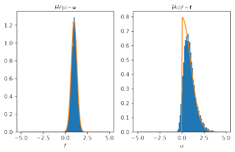
- [§4.2–4.3 and §5] The numerical evidence is qualitative. There are no error bars, no comparisons with existing conditional normalizing flows or direct inversion baselines, and no quantitative metrics for posterior sample quality. The statement in §5 that the construction has 'improved conditioning' is supported only by one toy condition-number plot. If the paper is to claim practical advantages, these need quantitative support; otherwise the claims should be moderated.
minor comments (4)
- [Remark 3.6] The claim that the triangular structure 'guarantees' a unique solution to the variational problems in Lemma 3.5 is too strong unless additional monotonicity and parameterization assumptions are imposed. Please qualify or remove.
- [Abstract and §4.1] Typos: 'in to one' should be 'into one'; 'with a a linear' should be 'with a linear'; 'Fischer information' should be 'Fisher information.'
- [§4.2] The map qF uses the sign function σ, which is not differentiable at 0. The density transformation via |∇qF^{-1}| is then not defined pointwise. Please clarify that the example is intended in a piecewise sense or use a smooth approximation.
- [Figures 6–8] Several figures lack axis labels and legends; adding these would improve interpretability, especially for the conditional-distribution and condition-number plots.
Circularity Check
No load-bearing circularity: the construction is a self-contained composition of triangular conditional maps; score 2 reflects only the presence of a minor, non-load-bearing self-citation.
full rationale
The central derivation is self-contained. Lemmas 3.3 and 3.4 show that lower- and upper-triangular maps qF and pF with qF#μX,Y = pF#μX,Y = μU,F yield conditional samplers Flike and Fpost by substitution. Equations (4)-(5) define S and R explicitly as compositions of these conditional maps, and Theorem 3.7 verifies S^{-1}=R and the push-forward identities by direct change-of-variables computation; the paper transparently states that i) and ii) hold by construction. No fitted parameter is renamed as a prediction: the numerical experiments are sanity checks or illustrations, not out-of-sample predictions forced by their training losses. The only self-citation appearing near the construction is [42], cited for 'Some experimental results using affine maps...', which is not used in the proof; the other self-citations are related-work mentions. The deterministic-likelihood/singular-measure restriction is a genuine assumption/invertibility limitation, but it is a scope condition, not a reduction of the claimed result to its own inputs. Hence no circular step is present; score 2 merely acknowledges a minor self-citation that is not load-bearing.
Assumptions & free parameters
free parameters (3)
- a,b in toy nonlinear map =
not reported
- Hermite polynomial total order =
4
- Affine normal parameters for MNIST =
mean/covariance estimated from training data
assumptions (3)
- domain assumption The joint distribution μU,F admits invertible lower-triangular and upper-triangular maps from a product reference measure μX⊗μY.
- standard math The reference measure is a product: μX,Y = μX⊗μY.
- standard math Existence of regular conditional distributions (disintegration).
Cite this review
Pith. "Pith review of An invertible generative model for forward and inverse problems." pith.science (2026). https://pith.science/paper/RIPXYMBY
@misc{pith2026250903910,
  author       = {Pith},
  title        = {Pith review of: An invertible generative model for forward and inverse problems},
  year         = {2026},
  howpublished = {\url{https://pith.science/paper/RIPXYMBY}},
  note         = {Machine review of arXiv:2509.03910}
}
read the original abstract
We formulate the inverse problem in a Bayesian framework and aim to train a generative model that allows us to simulate (i.e., sample from the likelihood) and do inference (i.e., sample from the posterior). We review the use of triangular normalizing flows for conditional sampling in this context and show how to combine two such triangular maps (an upper and a lower one) in to one invertible mapping that can be used for simulation and inference. We work out several useful properties of this invertible generative model and propose a possible training loss for training the map directly. We illustrate the workings of this new approach to conditional generative modeling numerically on a few stylized examples.
Figures


Figures from the paper (10 more)




Forward citations
Cited by 1 Pith paper
-
A Distributionally Robust Framework for Learned Reconstructions in Inverse Problems
Introduces structured DRO for learned inverse problem reconstructions with ambiguity sets aligned to the forward operator, yielding explicit dual representations and a worst-case bound that induces Tikhonov regulariza...
Reference graph
Works this paper leans on
-
[1]
Jonas Adler and Ozan ¨Oktem. Deep bayesian inversion. arXiv preprint arXiv:1811.05910, 2018
arXiv 2018
-
[2]
Learned primal-dual reconstruction
Jonas Adler and Ozan ¨Oktem. Learned primal-dual reconstruction. IEEE transactions on medical imaging , 37(6):1322–1332, 2018
work page 2018
-
[3]
Stochastic interpolants: A unifying framework for flows and diffusions
Michael S Albergo, Nicholas M Boffi, and Eric Vanden-Eijnden. Stochastic interpolants: A unifying framework for flows and diffusions. arXiv preprint arXiv:2303.08797, 2023
arXiv 2023
-
[4]
Nick Alger, Tucker Hartland, Noemi Petra, and Omar Ghattas. Point spread function approximation of high-rank hessians with locally supported nonneg- ative integral kernels. SIAM Journal on Scientific Computing , 46(3):A1658– A1689, 2024
work page 2024
-
[5]
Analyzing inverse problems with invertible neural networks
Lynton Ardizzone, Jakob Kruse, Sebastian J Wirkert, Daniel Rahner, Eric W Pellegrini, Ralf S Klessen, Lena Maier-Hein, Carsten Rother, and Ullrich K¨ othe. Analyzing inverse problems with invertible neural networks. CoRR, 2018
work page 2018
-
[6]
Solving inverse problems using data-driven models
Simon Arridge, Peter Maass, Ozan ¨Oktem, and Carola-Bibiane Sch¨ onlieb. Solving inverse problems using data-driven models. Acta Numerica, 28:1–174, 2019
2019
-
[7]
CAFLOW: Conditional autoregressive flows
Georgios Batzolis, Marcello Carioni, Christian Etmann, Soroosh Afyouni, Zoe Kourtzi, and Carola-Bibiane Sch¨ onlieb. CAFLOW: Conditional autoregressive flows. Foundations of Data Science , 6(4):553–583, 2024
work page 2024
-
[8]
Conditional image generation with score-based diffusion models
Georgios Batzolis, Jan Stanczuk, Carola-Bibiane Sch¨ onlieb, and Christian Et- mann. Conditional image generation with score-based diffusion models. arXiv preprint arXiv:2111.13606, 2021
arXiv 2021
Show all 45 references
-
[9]
Invertible residual networks
Jens Behrmann, Will Grathwohl, Ricky TQ Chen, David Duvenaud, and J¨ orn- Henrik Jacobsen. Invertible residual networks. In International conference on machine learning, pages 573–582. PMLR, 2019
2019
-
[10]
The promises and pit- falls of stochastic gradient langevin dynamics
Nicolas Brosse, Alain Durmus, and Eric Moulines. The promises and pit- falls of stochastic gradient langevin dynamics. In S. Bengio, H. Wallach, H. Larochelle, K. Grauman, N. Cesa-Bianchi, and R. Garnett, editors, Ad- vances in Neural Information Processing Systems , volume 31...
2018
-
[11]
Un- supervised approaches based on optimal transport and convex analysis for inverse problems in imaging
Marcello Carioni, Subhadip Mukherjee, Hong Ye Tan, and Junqi Tang. Un- supervised approaches based on optimal transport and convex analysis for inverse problems in imaging. In Data-driven Models in Inverse Problems . Walter de Gruyter GmbH & Co. KG, 2024
2024
-
[12]
Ricky T. Q. Chen, Yulia Rubanova, Jesse Bettencourt, and David K Du- venaud. Neural ordinary differential equations. In S. Bengio, H. Wallach, H. Larochelle, K. Grauman, N. Cesa-Bianchi, and R. Garnett, editors, Ad- vances in Neural Information Processing Systems , volume 31. ...
2018
-
[13]
Density estimation using real NVP
Laurent Dinh, Jascha Sohl-Dickstein, and Samy Bengio. Density estimation using real NVP. In International Conference on Learning Representations , 2017
2017
-
[14]
Deep equilibrium architec- tures for inverse problems in imaging
Davis Gilton, Gregory Ongie, and Rebecca Willett. Deep equilibrium architec- tures for inverse problems in imaging. IEEE Transactions on Computational Imaging, 7:1123–1133, 2021
2021
-
[15]
Generative adver- sarial networks
Ian Goodfellow, Jean Pouget-Abadie, Mehdi Mirza, Bing Xu, David Warde- Farley, Sherjil Ozair, Aaron Courville, and Yoshua Bengio. Generative adver- sarial networks. Communications of the ACM , 63(11):139–144, 2020
2020
-
[16]
Image restoration
Bahadir Gunturk and Xin Li. Image restoration. CRC Press, 2018
2018
-
[17]
Stochastic normal- izing flows for inverse problems: A markov chains viewpoint
Paul Hagemann, Johannes Hertrich, and Gabriele Steidl. Stochastic normal- izing flows for inverse problems: A markov chains viewpoint. SIAM/ASA Journal on Uncertainty Quantification , 10(3):1162–1190, 2022
2022
-
[18]
Computed tomography: algorithms, insight, and just enough theory
Per Christian Hansen, Jakob Jørgensen, and William RB Lionheart. Computed tomography: algorithms, insight, and just enough theory . SIAM, 2021
2021
-
[19]
Universal approximation property of invertible neural networks
Isao Ishikawa, Takeshi Teshima, Koichi Tojo, Kenta Oono, Masahiro Ikeda, and Masashi Sugiyama. Universal approximation property of invertible neural networks. Journal of Machine Learning Research , 24(287):1–68, 2023
2023
-
[20]
Deep convolutional neural network for inverse problems in imaging
Kyong Hwan Jin, Michael T McCann, Emmanuel Froustey, and Michael Unser. Deep convolutional neural network for inverse problems in imaging. IEEE transactions on image processing , 26(9):4509–4522, 2017
2017
-
[21]
A plug-and-play priors approach for solving nonlinear imaging inverse problems
Ulugbek S Kamilov, Hassan Mansour, and Brendt Wohlberg. A plug-and-play priors approach for solving nonlinear imaging inverse problems. IEEE Signal Processing Letters, 24(12):1872–1876, 2017
2017
-
[22]
Auto-encoding variational bayes
Diederik P Kingma and Max Welling. Auto-encoding variational bayes. arXiv preprint arXiv:1312.6114, 2013
2013 arXiv
-
[23]
Glow: Generative flow with invertible 1x1 convolutions
Durk P Kingma and Prafulla Dhariwal. Glow: Generative flow with invertible 1x1 convolutions. In S. Bengio, H. Wallach, H. Larochelle, K. Grauman, N. Cesa-Bianchi, and R. Garnett, editors, Advances in Neural Information Processing Systems, volume 31. Curran Associates, Inc., 2018
2018
-
[24]
Improved variational inference with inverse autoregressive flow
Durk P Kingma, Tim Salimans, Rafal Jozefowicz, Xi Chen, Ilya Sutskever, and Max Welling. Improved variational inference with inverse autoregressive flow. Advances in neural information processing systems , 29, 2016
2016
-
[25]
Prince, and Marcus A
Ivan Kobyzev, Simon J.D. Prince, and Marcus A. Brubaker. Normalizing Flows: An Introduction and Review of Current Methods. IEEE Transactions on Pattern Analysis and Machine Intelligence , 43(11):3964–3979, 2021
2021
-
[26]
Sr- flow: Learning the super-resolution space with normalizing flow
Andreas Lugmayr, Martin Danelljan, Luc Van Gool, and Radu Timofte. Sr- flow: Learning the super-resolution space with normalizing flow. In European conference on computer vision , pages 715–732. Springer, 2020
2020
-
[27]
Sam- pling via measure transport: An introduction
Youssef Marzouk, Tarek Moselhy, Matthew Parno, and Alessio Spantini. Sam- pling via measure transport: An introduction. Handbook of Uncertainty Quan- tification, pages 785–825, 2017. 21
2017
-
[28]
Conditional generative adversarial nets
Mehdi Mirza and Simon Osindero. Conditional generative adversarial nets. arXiv preprint arXiv:1411.1784 , 2014
2014 arXiv
-
[29]
VISCOS flows: Variational schur conditional sampling with normalizing flows, 2022
Vincent Moens, Aivar Sootla, Haitham Bou Ammar, and Jun Wang. VISCOS flows: Variational schur conditional sampling with normalizing flows, 2022
2022
-
[30]
Algorithm unrolling: Inter- pretable, efficient deep learning for signal and image processing
Vishal Monga, Yuelong Li, and Yonina C Eldar. Algorithm unrolling: Inter- pretable, efficient deep learning for signal and image processing. IEEE Signal Processing Magazine, 38(2):18–44, 2021
2021
-
[31]
Monotone Parameterization Toolbkit (MParT),
MParT Development Team. Monotone Parameterization Toolbkit (MParT),
-
[32]
End-to-end reconstruction meets data-driven regularization for inverse problems
Subhadip Mukherjee, Marcello Carioni, Ozan ¨Oktem, and Carola-Bibiane Sch¨ onlieb. End-to-end reconstruction meets data-driven regularization for inverse problems. Advances in Neural Information Processing Systems , 34:21413–21425, 2021
2021
-
[33]
Aspire: iterative amortized posterior inference for bayesian inverse problems
Rafael Orozco, Ali Siahkoohi, Mathias Louboutin, and Felix J Herrmann. Aspire: iterative amortized posterior inference for bayesian inverse problems. Inverse Problems, 41(4):045001, 2025
2025
-
[34]
Sinkhorn autoencoders
Giorgio Patrini, Rianne Van den Berg, Patrick Forre, Marcello Carioni, Samarth Bhargav, Max Welling, Tim Genewein, and Frank Nielsen. Sinkhorn autoencoders. In Uncertainty in Artificial Intelligence, pages 733–743. PMLR, 2020
2020
-
[35]
Radev, Ulf K
Stefan T. Radev, Ulf K. Mertens, Andreas Voss, Lynton Ardizzone, and Ullrich Kothe. BayesFlow: learning complex stochastic models with invertible neural networks. IEEE Transactions on Neural Networks and Learning Systems , 33(4):1452–1466, April 2022
2022
-
[36]
Radev, Marvin Schmitt, Valentin Pratz, Umberto Picchini, Ull- rich K¨ othe, and Paul-Christian B¨ urkner
Stefan T. Radev, Marvin Schmitt, Valentin Pratz, Umberto Picchini, Ull- rich K¨ othe, and Paul-Christian B¨ urkner. Jana: jointly amortized neural ap- proximation of complex bayesian models. In Proceedings of the Thirty-ninth Conference on Uncertainty in Artificial Intelligenc...
2023
-
[37]
Autore- gressive denoising diffusion models for multivariate probabilistic time series forecasting
Kashif Rasul, Calvin Seward, Ingmar Schuster, and Roland Vollgraf. Autore- gressive denoising diffusion models for multivariate probabilistic time series forecasting. In International conference on machine learning , pages 8857–
-
[38]
The little engine that could: Regularization by denoising (red)
Yaniv Romano, Michael Elad, and Peyman Milanfar. The little engine that could: Regularization by denoising (red). SIAM journal on imaging sciences , 10(4):1804–1844, 2017
2017
-
[39]
Variational methods in imaging , volume 167
Otmar Scherzer, Markus Grasmair, Harald Grossauer, Markus Haltmeier, and Frank Lenzen. Variational methods in imaging , volume 167. Springer, 2009
2009
-
[40]
Score-based generative modeling through stochastic differential equations
Yang Song, Jascha Sohl-Dickstein, Diederik P Kingma, Abhishek Kumar, Stefano Ermon, and Ben Poole. Score-based generative modeling through stochastic differential equations. arXiv preprint arXiv:2011.13456 , 2020. 22
2011 arXiv
-
[41]
Inverse Problem Theory and Methods for Model Parameter Estimation
Albert Tarantola. Inverse Problem Theory and Methods for Model Parameter Estimation. Society for Industrial and Applied Mathematics, 2005
2005
-
[42]
The reversible simulator – a data-driven approach for solving forward and inverse problems
Tristan van Leeuwen. The reversible simulator – a data-driven approach for solving forward and inverse problems. In Applications of Mathematics in Sciences, Engineering, and Economics , Springer Proceedings in Mathematics & Statistics, 2025
2025
-
[43]
Learning likelihoods with conditional normalizing flows
Christina Winkler, Daniel Worrall, Emiel Hoogeboom, and Max Welling. Learning likelihoods with conditional normalizing flows. arXiv preprint arXiv:1912.00042, 2019
1912 arXiv
-
[44]
Stochastic normalizing flows
Hao Wu, Jonas K¨ ohler, and Frank No´ e. Stochastic normalizing flows. Ad- vances in neural information processing systems , 33:5933–5944, 2020
2020
-
[45]
Image reconstruction by domain-transform manifold learning
Bo Zhu, Jeremiah Z Liu, Stephen F Cauley, Bruce R Rosen, and Matthew S Rosen. Image reconstruction by domain-transform manifold learning. Nature, 555(7697):487–492, 2018. 23
2018
Reviewed August 5, 2026 · model on record in the stance chip above.
Discussion (0). Sign in to comment.