REVIEW 3 major objections 5 minor 56 references
Scaling Collapse Reveals Universal Dynamics in Compute-Optimally Trained Neural Networks
T0 review · 3 major / 5 minor · reviewed 2026-08-06 · deepseek-v4-flash
Pith's one-line read Entire loss curves of compute-optimally trained networks collapse onto one universal shape.
desk verdict A real and novel empirical phenomenon—loss-curve collapse and supercollapse in compute-optimal training—honestly quantified, but with a soft spot in the L0-fitting circularity that needs independent validation before the universality claim is settled. read the letter →
The pith
A machine-rendered reading of the paper's core claim, the machinery that carries it, and where it could break.
The reading
What carries the argument
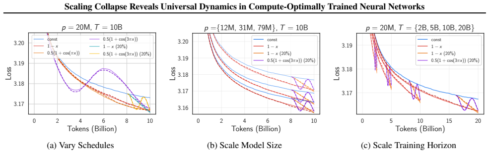
The central object is the affine normalization of Eq. (1), $\ell(x, p, \omega) = \left(L(x t^\star(p), p, \omega) - L_0\right)/\left(L(t^\star(p), p, \omega) - L_0\right)$, which maps every model's loss curve into the unit square in reducible loss versus normalized compute. The argument has three load-bearing pieces: (1) the sum-of-power-laws ansatz $L = L_0 + t^{-\mu} + p^{-\nu}$, which at the compute-optimal horizon $t^\star \propto p^{\nu/\mu}$ makes the normalized curve exactly independent of $p$; (2) a quadratic-SDE model of SGD noise in gradient-flow time, which gives the approximate loss shift $\delta L \approx \alpha\, \delta\eta(\tau)\, \mathrm{Tr}(\Sigma'(\tau))$ and predicts that schedule-induced deformations are shared across model sizes because $\mathrm{Tr}(\Sigma)/L$ depends only on normalized compute; and (3) a first-order variance computation showing the normalized-curve variance obeys $\Delta^2 \propto \eta(\tau)(1 - \hat{\tau})$ near the end of training, explaining why learning-rate decay produces supercollapse.
What would settle it
Train a compute-optimal scaling ladder on a task where the irreducible loss can be pinned down independently of the collapse analysis—for example, by measuring the loss of a very large model trained for a very long time, or by injecting label noise so the Bayes error is known—and check whether curves from different sizes still collapse under Eq. (1) when that independently fixed $L_0$ is subtracted. A second check is to test whether the predicted scaling $\Delta^2 \propto \eta(\tau)(1 - \hat{\tau})$ holds for schedules the paper did not try, such as exponential or stepwise decay; failure of either check would indicate that the universality is fit-dependent.
Extended reading notes
Core claim
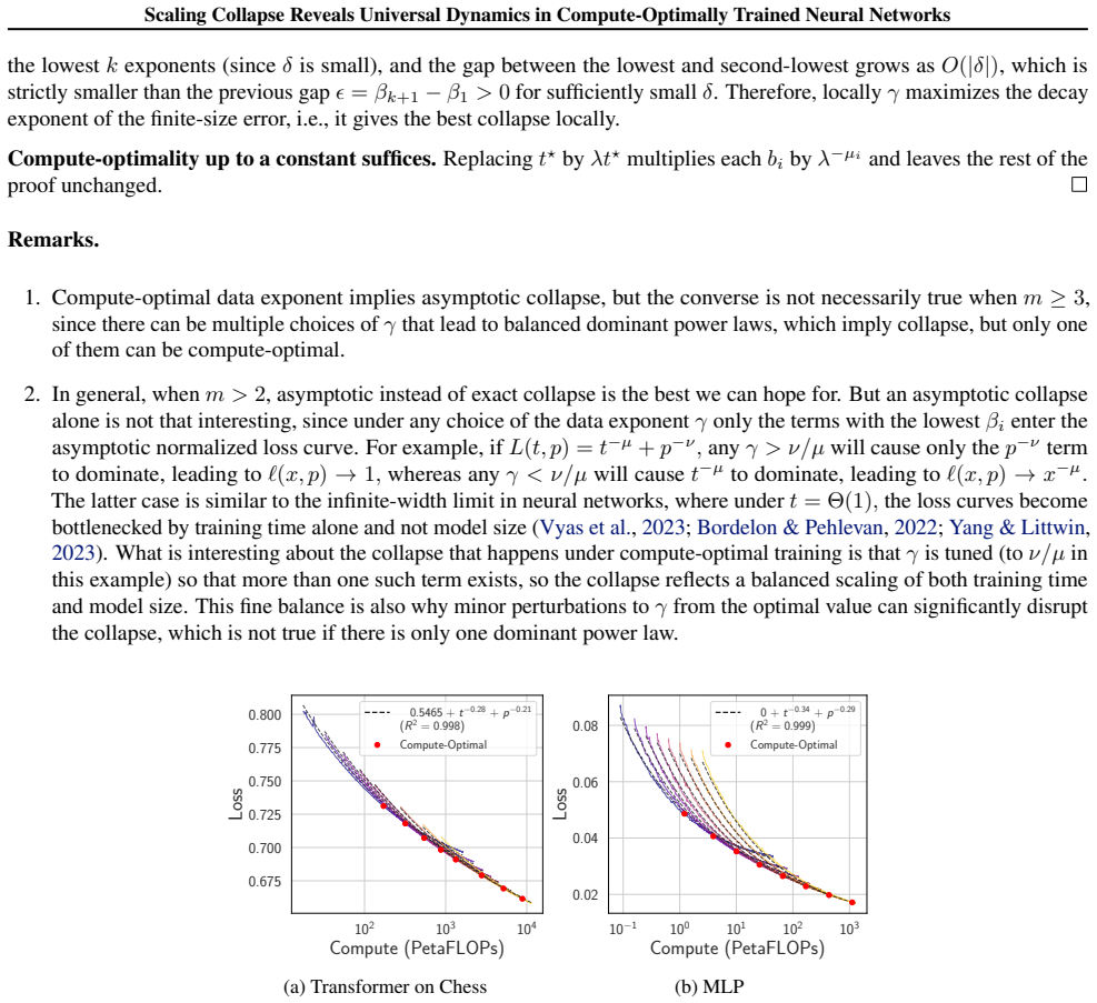
After subtracting a fitted irreducible loss $L_0$ and rescaling so that final compute and final reducible loss are both $1$, the loss curves $L(t, p, \omega)$ of compute-optimally trained models satisfy, to high precision, a size-independent identity: the normalized curve $\ell(x)$ is the same function of normalized compute $x = t/t^\star(p)$ for all model sizes $p$ under a fixed learning-rate schedule. For loss functions of the form $L = L_0 + t^{-\mu} + p^{-\nu}$, this identity is exact at the compute-optimal horizon $t^\star(p) \propto p^{\nu/\mu}$, giving $\ell(x) = (r x^{-\mu} + 1)/(r+1)$ with $r = \nu/\mu$, independent of $p$ (Eq. 7). The identity persists across learning-rate schedules because a quadratic-noise model of SGD predicts that schedule-induced deformations depend on the product of the instantaneous learning rate and the gradient-covariance trace, and the ratio $\mathrm{Tr}(\Sigma)/L$ is empirically a function of normalized compute alone. Learning-rate decay makes the collapse ``super'': the variance of the normalized curves scales as $\eta(\tau)(1 - \hat{\tau})$, so normalizing by the realized final loss cancels most of the seed noise, pushing the collapse below the single-trajectory noise floor. The paper argues that when the data exponent or parameterization is scaled suboptimally, the collapse breaks, making it a practical indicator of good scaling.
Load-bearing premise
The load-bearing premise is that the fitted irreducible loss $L_0$ and the fitted data exponent $\gamma$ correctly describe the asymptotic scaling; both are estimated from the very loss curves whose collapse is then reported, so a misestimated $L_0$ or $\gamma$ could make the universal curve and supercollapse partly artifacts of the fitting procedure.
Editorial extensions
If this is right
- Loss-curve prediction becomes a scaling-law problem: for a new model size, the entire compute-optimal loss trajectory can be predicted from the universal curve and the fitted $L_0$, without training to completion.
- The collapse can be measured cheaply and used to validate whether hyperparameters such as learning-rate parameterization and the data exponent are scaled correctly, since suboptimal choices break the collapse even when final losses look similar.
- The supercollapse criterion gives a noise-floor-limited comparison of models across scales, so single-seed training runs may suffice to detect scaling inconsistencies that currently require many seeds.
- The variance law $\Delta^2 \propto \eta(\tau)(1 - \hat{\tau})$ makes a quantitative, schedule-specific prediction for how quickly the collapse should improve as learning rate is decayed, which is testable in new settings.
- The result suggests a joint scaling limit in model size and training time that preserves consistency throughout training, complementing infinite-width limits that diverge at late times.
Reading between the lines
- One testable extension, not pursued in the paper, is to use the collapse deviation itself as an objective: tune the data exponent $\gamma$, parameterization, and schedule to maximize collapse tightness instead of fitting sparse final-loss power laws.
- This suggests that the ratio $\mathrm{Tr}(\Sigma)/L$, if universal in normalized compute, could let practitioners measure gradient-noise statistics on small models and transfer them to large models at matched normalized compute, giving a budget-free way to predict schedule effects.
- The authors compare their phenomenon to renormalization-group universality; if that analogy is substantive, collapse should persist to larger scales and new architectures, and deviations from collapse would be interpretable as relevant scaling variables that must be tuned.
- The control-variate view of normalization by the realized final loss suggests that other late-time observables, such as gradient norms, could be used to denoise and collapse different training statistics, not just the loss.
Editorial analysis
A structured set of objections, weighed in public.
Referee Report
Summary. This paper reports a scaling phenomenon in compute-optimally trained networks: after normalizing training compute by the estimated compute-optimal horizon t*(p) ∝ p^γ and normalizing the reducible loss (total loss minus a fitted irreducible offset L0) by the final reducible loss at that horizon, loss curves from models spanning roughly an order of magnitude in width collapse onto a single schedule-dependent universal curve (Eq. 1; Figs. 1–3). With learning-rate decay, the cross-size collapse deviation Δ falls below the per-seed noise floor σ for a substantial fraction of training, a phenomenon the authors call supercollapse (Fig. 1c). The theoretical component has three parts: (i) for losses of the form L0 + t^{-μ} + p^{-ν}, compute-optimal allocation makes the normalized curve exactly p-independent (Eq. 7); (ii) a theorem (E.1) states that full collapse forces a power-law Pareto frontier; and (iii) a quadratic/SDE model of schedule-dependent SGD noise predicts loss curves across schedules, model sizes, and horizons with a single fitted constant α (Eqs. 16–18; Fig. 6) and predicts Δ² ∝ η(τ̂)(1 − τ̂) during decay (Eq. 24; Fig. 8). Experiments include transformers on CIFAR-5M and chess, MLPs on a power-law-spectrum regression task, width- and depth-scaling ladders, and negative controls (constant-LR parameterization; wrong data exponent) showing that collapse breaks under suboptimal scaling choices.
Significance. If the main claim holds, the paper is significant: it extends scaling laws from statements about final losses to statements about the entire training trajectory, and it provides evidence for a joint limit in which model size and training time grow together under compute-optimal allocation while preserving dynamical consistency across sizes, in contrast to the divergence found in fixed-horizon infinite-width limits (Vyas et al., 2023, cited). The empirical core is unusually well quantified for a scaling-laws paper: collapse deviation is always compared with a per-seed noise floor (Eqs. 2–3); collapse is shown to break under both wrong parameterization and wrong data exponent (Fig. 4), giving the claim falsifiable content; the MLP setup has known L0 = 0 as a positive control; multiple seeds are used; and the code is released. The schedule-prediction model's success across schedules, widths, and horizons with a single fitted α (0.21, close to the theoretical 1/4) is a genuine predictive achievement (Fig. 6, Appendix I).
major comments (3)
- [§2.2–2.4, Eq. (1), Fig. 2, Appendix C] The collapse observable is not a raw quantity: both the offset L0 subtracted in Eq. (1) and the horizon t*(p) ∝ p^γ that sets the normalized-compute axis are fitted to the same loss curves whose collapse is then asserted. Figure 2 shows that shifting L0 by only −0.012 or +0.008 from the fitted value 3.132 destroys the collapse, yet the paper reports no uncertainty for L0 or γ, and two separate fits on the same CIFAR-5M data give L0 = 3.132 (Fig. 1a) and L0 = 3.134 (Fig. 5a). Because the least-squares fit of L0 + ac^{-b} uses a small number of effectively independent Pareto-frontier points estimated from only 5 seeds, the plausible uncertainty in L0 may be comparable to the ±0.01 sensitivity scale, in which case part of the observed collapse could be an artifact of choosing L0 to make the frontier a power law (which Theorem E.1 shows is necessary for collapse). The nontrivial content is full-curve collapse over x ∈ (0,1], since the frontier fit constrains only final losses and the slope at x = 1; to support that claim, the authors should report bootstrap or seed-subsample uncertainties on (L0, γ, a, b), re-evaluate Δ(x) for L0 at the extremes of that uncertainty, and perform a held-out check in which L0 and γ are fit on a subset of the scaling ladder and the collapse is measured on the complementary subset. The MLP positive control (known L0 = 0) and the Fig. 4 sensitivity experiments are good first steps, but they do not resolve the fitting-circularity concern for the headline transformer results.
- [Appendix E (Theorem E.1 and its Remark), §3.1] Section 3.1 presents the power-law Pareto frontier as necessary for collapse and uses this to justify the choice L̂ = L0, but the proof requires the compute-optimal point to be interior to each loss curve. The Remark appended to Theorem E.1 concedes that this condition fails for schedules that reach η = 0 after finitely many steps, which are exactly the schedules on which the headline supercollapse results (Figs. 1b–c and 4) are demonstrated. As written, the theorem is formally established for the constant-LR family used to estimate t*(p), but its necessity claim is not established for the decaying-schedule runs, and its sufficiency direction yields only first-order collapse rather than full-curve supercollapse. The explanation of supercollapse therefore rests on the empirical noise model of Section 3.3 rather than on Theorem E.1, which is acceptable, but the 'necessary' narrative in Section 3.1 should be restricted to the setting where the hypotheses hold, or the proof should be extended to boundary-optimal schedules; the Remark's caveat should also be surfaced in the main text rather than only in the appendix.
- [§3.1, Eq. (7), Fig. 5, Fig. 10d] The theoretical derivation's main deliverable is an explicit universal curve ℓ(x) = (r x^{-μ} + 1)/(r + 1), and Fig. 5a reports a fit of L0 + t^{-μ} + p^{-ν} to the CIFAR-5M loss surface with L0 = 3.134, μ = 0.41, and ν = 0.37 (R² = 0.999). The paper never overlays this predicted curve on the empirically collapsed constant-LR curves of Fig. 3, nor does it report the deviation between the predicted and observed normalized curves relative to the seed noise floor. In addition, the theory predicts the data exponent γ = ν/μ ≈ 0.90, which differs from the empirically estimated γ = 0.96 (Fig. 10d) without any comment on the discrepancy. Adding the predicted-curve overlay (and an analogous check for the schedule-transferred prediction of Eq. (21)) would test the quantitative content of the claimed universality rather than only its cross-size aspect, and would also help bound the circularity raised in the first major comment, since the same fitted exponents define the normalization.
minor comments (5)
- [§2.4, Eqs. (2)–(3), Fig. 1c] The noise floor σ(x, p) is defined per model size in Eq. (3), but Fig. 1c plots a single noise-floor curve and compares it with the p-averaged Δ(x); the paper should state whether the plotted floor is the mean, median, or maximum over p and should define the comparison criterion behind the claim Δ(x) < σ.
- [§3.2.2, Eqs. (16)–(18)] The closed-form prediction (1 − αh(x)δη(τ,p))^{-1} appears in Eq. (18) without derivation from the linearized expression in Eq. (16); a one-sentence geometric-series justification and its regime of validity (small αhδη) would prevent confusion.
- [§3.2.2, Fig. 6, Appendix A] The schedule-prediction experiments on CIFAR-5M use a different configuration from the collapse experiments (different codebase, base width, initialization, learning rate, and batch size, as described in Appendix A); the main text should flag this so readers do not treat Fig. 6 as validating the exact runs of Fig. 1.
- [Appendix C, Appendix G, Figs. 1a and 5a] Presentation issues: the typos 'origianlly' (Appendix C) and 'dervie' (Appendix G) should be fixed, and the two fitted CIFAR-5M values L0 = 3.132 (Fig. 1a) and L0 = 3.134 (Fig. 5a) should be reconciled or explicitly explained in the text.
- [§3.3, Fig. 8] The predicted scaling in Fig. 8 is stated in terms of normalized gradient-flow time τ̂ while the rest of the paper uses normalized compute x = t/t⋆(p); a sentence relating the two normalizations would let the reader compare Fig. 8 directly with Fig. 1c.
Circularity Check
The universal-curve and schedule-prediction claims are partly self-referential because the normalizing offset L0 and the schedule coefficient α are fitted on the same curves used as evidence, but full-curve collapse and supercollapse remain empirically nontrivial.
-
fitted input called prediction
[Sections 2.2-2.3, Eq. (1), Figure 2]
"Using the best-fit L0, we define the reducible loss curve L(t, p, ω) = L(t, p, ω) − L0. ... We set ˆL = L0 to subtract the estimated irreducible loss ... We found setting ˆL = L0 achieves the best collapse (Figure 2)."
The central observable ℓ(x,p,ω) whose p-independence is claimed as universality is constructed with a fitted offset L0 and a fitted compute axis t*(p) estimated from the same loss curves. Figure 2 shows collapse quality is maximized at the fitted L0, so the reported 'best collapse' is partly selected by the fit rather than measured independently. The paper gives no error bars on L0 or γ and no held-out model/schedule validation. However, one scalar per task does not by itself force the entire normalized curve to be p-independent, so the reduction is partial.
-
fitted input called prediction
[Section 3.2.2, Eqs. (16)-(18), Figure 6]
"where α is a shared hyperparameter. We find a single α = 0.21 fits the target loss curves surprisingly well across schedules, model sizes, and training horizons."
The loss curves presented as 'predictions' (Figure 1e, Figure 6) are generated with a coefficient α fitted to those same curves; the theory's derived value 1/4 is replaced by the free parameter α (0.21 for CIFAR-5M, 0.26 for MLP). Thus the quantitative agreement is a one-parameter fit rather than an ab initio prediction. The schedule-dependent shape via δη(τ)Tr(Σ'(τ)) is non-trivial and not implied by the fit alone, which limits the severity.
full rationale
The paper's core Section 3.1 derivation is not circular: given an exact sum-of-power-laws loss with power-law Pareto frontier, Eq. (7) algebraically cancels p, and Theorem E.1/F provide a genuine necessary/sufficient analysis under stated assumptions. The main self-referential content is (i) the affine normalization in Eq. (1) uses L0 and t*(p) estimated from the very curves whose collapse is claimed, with Figure 2 showing collapse peaks at the fitted offset; and (ii) the schedule-prediction model uses a fitted coefficient α in place of the derived 1/4. No load-bearing uniqueness theorem is imported from the authors' own previous work: cites to Paquette et al. (2024b) and Agarwala & Pennington (2024) are motivational or auxiliary, and the key empirical checks (Figures 7, 14) are independent measurements. The MLP experiment with known L0=0 is a useful positive control, so the central observation has independent content despite the fitted normalization. The paper itself flags a nontrivial limitation in Theorem E.1's Remark: the interior compute-optimality assumption can fail for schedules that reach η=0 after finitely many steps, exactly the schedules where supercollapse is claimed; this weakens the necessity proof but is not a circularity. Overall: partial circularity through fitted inputs, not a by-construction equivalence, so score 4.
Assumptions & free parameters
free parameters (6)
- L0 (irreducible loss offset) =
3.132 (CIFAR-5M), 0.545 (chess), fitted per scaling ladder
- a, b (scaling law constants) =
a=0.154, b=0.191 (CIFAR-5M, Figure 1a)
- gamma (data exponent) =
0.96 (CIFAR-5M), 1.04 (MLP), 1.02 (chess optimal), 1.2 (deliberately suboptimal)
- kappa (prefactor in c*(p)) =
5.34e5 (CIFAR-5M), 1.35e6 (MLP)
- alpha (noise model constant) =
0.21 (CIFAR-5M), 0.26 (MLP)
- sum-of-power-law exponents mu, nu =
CIFAR-5M t^{-0.41}+p^{-0.37}; chess t^{-0.28}+p^{-0.21}; MLP t^{-0.34}+p^{-0.29}
assumptions (6)
- domain assumption Compute-optimal loss curves follow the sum-of-power-laws form L(t,p) = L0 + t^{-mu} + p^{-nu}, generalized to Eq (8).
- domain assumption Gradient noise is modeled by the SDE dw/dtau = -(grad L(w) + Sigma^{1/2}(w) xi(tau)) with E[xi xi'] = eta(tau) delta, and the noise-induced loss shift is approximately (1/4) eta(tau) Tr(Sigma-bar(tau)) in the slow-variation, late-time limit.
- domain assumption The compute-optimal horizon t*(p) estimated under a constant learning rate transfers to other schedules up to a constant factor.
- domain assumption The trace universality Tr(Sigma(xt*(p)))/L(xt*(p)) approximately equals h(x), independent of model size p for a given schedule.
- standard math The envelope theorem applies to the compute-optimal point of each loss curve, requiring interior optima.
- domain assumption muP (maximal update parameterization) supplies correctly width-scaled initialization and learning rates, so training dynamics are comparable across widths.
invented entities (1)
-
Universal collapse curve l(x) and the compute-optimal joint scaling limit
Cite this review
Pith. "Pith review of Scaling Collapse Reveals Universal Dynamics in Compute-Optimally Trained Neural Networks." pith.science (2026). https://pith.science/paper/RKC6QSF3
@misc{pith2026250702119,
  author       = {Pith},
  title        = {Pith review of: Scaling Collapse Reveals Universal Dynamics in Compute-Optimally Trained Neural Networks},
  year         = {2026},
  howpublished = {\url{https://pith.science/paper/RKC6QSF3}},
  note         = {Machine review of arXiv:2507.02119}
}
read the original abstract
What scaling limits govern neural network training dynamics when model size and training time grow in tandem? We show that despite the complex interactions between architecture, training algorithms, and data, compute-optimally trained models exhibit a remarkably precise universality. Specifically, loss curves from models of varying sizes collapse onto a single universal curve when training compute and loss are normalized to unity at the end of training. With learning rate decay, the collapse becomes so tight that differences in the normalized curves across models fall below the noise floor of individual loss curves across random seeds, a phenomenon we term supercollapse. We observe supercollapse across learning rate schedules, datasets, and architectures, including transformers trained on next-token prediction, and find it breaks down when hyperparameters are scaled suboptimally, providing a precise and practical indicator of good scaling. We explain these phenomena by connecting collapse to the power-law structure in typical neural scaling laws, and analyzing a simple yet surprisingly effective model of SGD noise dynamics that accurately predicts loss curves across various learning rate schedules and quantitatively explains the origin of supercollapse.
Figures


Figures from the paper (11 more)






Reference graph
Works this paper leans on
-
[1]
L., Almeida, D., Altenschmidt, J., Altman, S., Anadkat, S., et al
Achiam, J., Adler, S., Agarwal, S., Ahmad, L., Akkaya, I., Aleman, F. L., Almeida, D., Altenschmidt, J., Altman, S., Anadkat, S., et al. Gpt-4 technical report. arXiv preprint arXiv:2303.08774, 2023
arXiv 2023
-
[2]
Agarwala, A. and Fisher, D. S. Adaptive walks on high-dimensional fitness landscapes and seascapes with distance-dependent statistics. Theoretical population biology, 130: 0 13--49, 2019
work page 2019
-
[3]
Agarwala, A. and Pennington, J. High dimensional analysis reveals conservative sharpening and a stochastic edge of stability, 2024. URL https://arxiv.org/abs/2404.19261
arXiv 2024
-
[4]
Power lines: Scaling laws for weight decay and batch size in llm pre-training
Bergsma, S., Dey, N., Gosal, G., Gray, G., Soboleva, D., and Hestness, J. Power lines: Scaling laws for weight decay and batch size in llm pre-training. arXiv preprint arXiv:2505.13738, 2025
arXiv 2025
-
[5]
Finite size scaling analysis of ising model block distribution functions
Binder, K. Finite size scaling analysis of ising model block distribution functions. Zeitschrift f \"u r Physik B Condensed Matter , 43: 0 119--140, 1981
work page 1981
-
[6]
Bordelon, B. and Pehlevan, C. Self-consistent dynamical field theory of kernel evolution in wide neural networks. Advances in Neural Information Processing Systems, 35: 0 32240--32256, 2022
work page 2022
-
[7]
B., Hanin, B., and Pehlevan, C
Bordelon, B., Noci, L., Li, M. B., Hanin, B., and Pehlevan, C. Depthwise hyperparameter transfer in residual networks: Dynamics and scaling limit. arXiv preprint arXiv:2309.16620, 2023
arXiv 2023
-
[8]
A dynamical model of neural scaling laws
Bordelon, B., Atanasov, A., and Pehlevan, C. A dynamical model of neural scaling laws. arXiv preprint arXiv:2402.01092, 2024 a
arXiv 2024
Show all 56 references
-
[9]
How feature learning can improve neural scaling laws
Bordelon, B., Atanasov, A., and Pehlevan, C. How feature learning can improve neural scaling laws. arXiv preprint arXiv:2409.17858, 2024 b
2024 arXiv
-
[10]
Infinite limits of multi-head transformer dynamics
Bordelon, B., Chaudhry, H., and Pehlevan, C. Infinite limits of multi-head transformer dynamics. Advances in Neural Information Processing Systems, 37: 0 35824--35878, 2024 c
2024
-
[11]
M., Kaur, S., Li, Y., Kolter, J
Cohen, J. M., Kaur, S., Li, Y., Kolter, J. Z., and Talwalkar, A. Gradient descent on neural networks typically occurs at the edge of stability. arXiv preprint arXiv:2103.00065, 2021
2021 arXiv
-
[12]
M., Ghorbani, B., Krishnan, S., Agarwal, N., Medapati, S., Badura, M., Suo, D., Cardoze, D., Nado, Z., Dahl, G
Cohen, J. M., Ghorbani, B., Krishnan, S., Agarwal, N., Medapati, S., Badura, M., Suo, D., Cardoze, D., Nado, Z., Dahl, G. E., et al. Adaptive gradient methods at the edge of stability. arXiv preprint arXiv:2207.14484, 2022
2022 arXiv
-
[13]
M., Damian, A., Talwalkar, A., Kolter, Z., and Lee, J
Cohen, J. M., Damian, A., Talwalkar, A., Kolter, Z., and Lee, J. D. Understanding optimization in deep learning with central flows. arXiv preprint arXiv:2410.24206, 2024
2024
-
[14]
Optimal learning rate schedules in high-dimensional non-convex optimization problems
d'Ascoli, S., Refinetti, M., and Biroli, G. Optimal learning rate schedules in high-dimensional non-convex optimization problems. arXiv preprint arXiv:2202.04509, 2022
2022 arXiv
-
[15]
C., Noci, L., Li, M., Bordelon, B., Bergsma, S., Pehlevan, C., Hanin, B., and Hestness, J
Dey, N., Zhang, B. C., Noci, L., Li, M., Bordelon, B., Bergsma, S., Pehlevan, C., Hanin, B., and Hestness, J. Don't be lazy: Completep enables compute-efficient deep transformers. arXiv preprint arXiv:2505.01618, 2025
2025
-
[16]
Kingma, J
Diederik P. Kingma, J. B. Adam: A Method for Stochastic Optimization . International Conference on Learning Representations (ICLR), 2015
2015
-
[17]
A., Novak, R., Liu, P
Everett, K., Xiao, L., Wortsman, M., Alemi, A. A., Novak, R., Liu, P. J., Gur, I., Sohl-Dickstein, J., Kaelbling, L. P., Lee, J., et al. Scaling exponents across parameterizations and optimizers. arXiv preprint arXiv:2407.05872, 2024
2024 arXiv
-
[18]
Fisher, D. S. Asexual evolution waves: fluctuations and universality. Journal of Statistical Mechanics: Theory and Experiment, 2013 0 (01): 0 P01011, 2013
2013
-
[19]
Monte Carlo methods in financial engineering, volume 53
Glasserman, P. Monte Carlo methods in financial engineering, volume 53. Springer, 2004
2004
-
[20]
and Fisher, D
Hallatschek, O. and Fisher, D. S. Acceleration of evolutionary spread by long-range dispersal. Proceedings of the National Academy of Sciences, 111 0 (46): 0 E4911--E4919, 2014
2014
-
[21]
and Gimpel, K
Hendrycks, D. and Gimpel, K. Gaussian Error Linear Units (GELUs) . Preprint arXiv 1606.08415, 2016
2016 arXiv
-
[22]
Hestness, J., Narang, S., Ardalani, N., Diamos, G., Jun, H., Kianinejad, H., Patwary, M. M. A., Yang, Y., and Zhou, Y. Deep learning scaling is predictable, empirically. arXiv preprint arXiv:1712.00409, 2017
2017 arXiv
-
[23]
Hoffmann, J., Borgeaud, S., Mensch, A., Buchatskaya, E., Cai, T., Rutherford, E., Casas, D. d. L., Hendricks, L. A., Welbl, J., Clark, A., et al. Training compute-optimal large language models. arXiv preprint arXiv:2203.15556, 2022
2022 arXiv
-
[24]
B., Chess, B., Child, R., Gray, S., Radford, A., Wu, J., and Amodei, D
Kaplan, J., McCandlish, S., Henighan, T., Brown, T. B., Chess, B., Child, R., Gray, S., Radford, A., Wu, J., and Amodei, D. Scaling laws for neural language models. arXiv preprint arXiv:2001.08361, 2020
2001 arXiv
-
[25]
F., Blundell, J
Levy, S. F., Blundell, J. R., Venkataram, S., Petrov, D. A., Fisher, D. S., and Sherlock, G. Quantitative evolutionary dynamics using high-resolution lineage tracking. Nature, 519 0 (7542): 0 181--186, 2015
2015
-
[26]
Stochastic modified equations and adaptive stochastic gradient algorithms
Li, Q., Tai, C., et al. Stochastic modified equations and adaptive stochastic gradient algorithms. In International Conference on Machine Learning, pp.\ 2101--2110. PMLR, 2017
2017
-
[27]
A multi-power law for loss curve prediction across learning rate schedules
Luo, K., Wen, H., Hu, S., Sun, Z., Liu, Z., Sun, M., Lyu, K., and Chen, W. A multi-power law for loss curve prediction across learning rate schedules. arXiv preprint arXiv:2503.12811, 2025
2025 arXiv
-
[28]
On the sdes and scaling rules for adaptive gradient algorithms
Malladi, S., Lyu, K., Panigrahi, A., and Arora, S. On the sdes and scaling rules for adaptive gradient algorithms. Advances in Neural Information Processing Systems, 35: 0 7697--7711, 2022
2022
-
[29]
and Pastur, L
Marchenko, V. and Pastur, L. A. Distribution of eigenvalues for some sets of random matrices. Mat. Sb.(NS), 72 0 (114): 0 4, 1967
1967
-
[30]
McCandlish, S., Kaplan, J., Amodei, D., and Team, O. D. An empirical model of large-batch training. arXiv preprint arXiv:1812.06162, 2018
2018 arXiv
-
[31]
Y., Singh, S., Bhatele, A., Goldblum, M., Panda, A., and Goldstein, T
McLeish, S., Kirchenbauer, J., Miller, D. Y., Singh, S., Bhatele, A., Goldblum, M., Panda, A., and Goldstein, T. Gemstones: A model suite for multi-faceted scaling laws. arXiv preprint arXiv:2502.06857, 2025
2025
-
[32]
The deep bootstrap framework: Good online learners are good offline generalizers
Nakkiran, P., Neyshabur, B., and Sedghi, H. The deep bootstrap framework: Good online learners are good offline generalizers. arXiv preprint arXiv:2010.08127, 2020
2010 arXiv
-
[33]
Super consistency of neural network landscapes and learning rate transfer
Noci, L., Meterez, A., Hofmann, T., and Orvieto, A. Super consistency of neural network landscapes and learning rate transfer. Advances in Neural Information Processing Systems, 37: 0 102696--102743, 2024
2024
-
[34]
Sgd in the large: Average-case analysis, asymptotics, and stepsize criticality
Paquette, C., Lee, K., Pedregosa, F., and Paquette, E. Sgd in the large: Average-case analysis, asymptotics, and stepsize criticality. In Conference on Learning Theory, pp.\ 3548--3626. PMLR, 2021
2021
-
[35]
Homogenization of sgd in high-dimensions: Exact dynamics and generalization properties
Paquette, C., Paquette, E., Adlam, B., and Pennington, J. Homogenization of sgd in high-dimensions: Exact dynamics and generalization properties. Mathematical Programming, pp.\ 1--90, 2024 a
2024
-
[36]
4+ 3 phases of compute-optimal neural scaling laws
Paquette, E., Paquette, C., Xiao, L., and Pennington, J. 4+ 3 phases of compute-optimal neural scaling laws. arXiv preprint arXiv:2405.15074, 2024 b
2024 arXiv
-
[37]
T., Agarwala, A., and Fisher, D
Pearce, M. T., Agarwala, A., and Fisher, D. S. Stabilization of extensive fine-scale diversity by ecologically driven spatiotemporal chaos. Proceedings of the National Academy of Sciences, 117 0 (25): 0 14572--14583, 2020
2020
-
[38]
and Song, J
Pearce, T. and Song, J. Reconciling kaplan and chinchilla scaling laws. arXiv preprint arXiv:2406.12907, 2024
2024 arXiv
-
[39]
J., Davison, M., Bhaya, D., and Fisher, D
Rosen, M. J., Davison, M., Bhaya, D., and Fisher, D. S. Fine-scale diversity and extensive recombination in a quasisexual bacterial population occupying a broad niche. Science, 348 0 (6238): 0 1019--1023, 2015
2015
-
[40]
The surprising agreement between convex optimization theory and learning-rate scheduling for large model training
Schaipp, F., H \"a gele, A., Taylor, A., Simsekli, U., and Bach, F. The surprising agreement between convex optimization theory and learning-rate scheduling for large model training. arXiv preprint arXiv:2501.18965, 2025
2025 arXiv
-
[41]
Ubiquitous abundance distribution of non-dominant plankton across the global ocean
Ser-Giacomi, E., Zinger, L., Malviya, S., De Vargas, C., Karsenti, E., Bowler, C., and De Monte, S. Ubiquitous abundance distribution of non-dominant plankton across the global ocean. Nature ecology & evolution, 2 0 (8): 0 1243--1249, 2018
2018
-
[42]
and Kaplan, J
Sharma, U. and Kaplan, J. Scaling laws from the data manifold dimension. Journal of Machine Learning Research, 23 0 (9): 0 1--34, 2022
2022
-
[43]
Tamai, K., Okubo, T., Duy, T. V. T., Natori, N., and Todo, S. Universal scaling laws of absorbing phase transitions in artificial deep neural networks. arXiv preprint arXiv:2307.02284, 2023
2023 arXiv
-
[44]
Scaling law with learning rate annealing
Tissue, H., Wang, V., and Wang, L. Scaling law with learning rate annealing. arXiv preprint arXiv:2408.11029, 2024
2024 arXiv
-
[45]
R., Geiler-Samerotte, K., H \'e rissant, L., Blundell, J
Venkataram, S., Dunn, B., Li, Y., Agarwala, A., Chang, J., Ebel, E. R., Geiler-Samerotte, K., H \'e rissant, L., Blundell, J. R., Levy, S. F., et al. Development of a comprehensive genotype-to-fitness map of adaptation-driving mutations in yeast. Cell, 166 0 (6): 0 1585--1596, 2016
2016
-
[46]
Feature-learning networks are consistent across widths at realistic scales
Vyas, N., Atanasov, A., Bordelon, B., Morwani, D., Sainathan, S., and Pehlevan, C. Feature-learning networks are consistent across widths at realistic scales. Advances in Neural Information Processing Systems, 36: 0 1036--1060, 2023
2023
-
[47]
and Aitchison, L
Wang, X. and Aitchison, L. How to set adamw's weight decay as you scale model and dataset size. arXiv preprint arXiv:2405.13698, 2024
2024 arXiv
-
[48]
Understanding warmup-stable-decay learning rates: A river valley loss landscape perspective
Wen, K., Li, Z., Wang, J., Hall, D., Liang, P., and Ma, T. Understanding warmup-stable-decay learning rates: A river valley loss landscape perspective. arXiv preprint arXiv:2410.05192, 2024
2024 arXiv
-
[49]
Wilson, K. G. Renormalization group and critical phenomena. i. renormalization group and the kadanoff scaling picture. Physical review B, 4 0 (9): 0 3174, 1971
1971
-
[50]
J., Xiao, L., Everett, K., Alemi, A., Adlam, B., Co-Reyes, J
Wortsman, M., Liu, P. J., Xiao, L., Everett, K., Alemi, A., Adlam, B., Co-Reyes, J. D., Gur, I., Kumar, A., Novak, R., et al. Small-scale proxies for large-scale transformer training instabilities. arXiv preprint arXiv:2309.14322, 2023
2023 arXiv
-
[51]
Rethinking conventional wisdom in machine learning: From generalization to scaling
Xiao, L. Rethinking conventional wisdom in machine learning: From generalization to scaling. arXiv preprint arXiv:2409.15156, 2024
2024 arXiv
-
[52]
and Hu, E
Yang, G. and Hu, E. J. Feature Learning in Infinite-Width Neural Networks . International Conference on Machine Learning (ICML), 2021
2021
-
[53]
and Littwin, E
Yang, G. and Littwin, E. Tensor Programs IVb: Adaptive Optimization in the Infinite-Width Limit . International Conference on Learning Representations (ICLR), 2023
2023
-
[54]
J., Babuschkin, I., Sidor, S., Liu, X., Farhi, D., Ryder, N., Pachocki, J., Chen, W., and Gao, J
Yang, G., Hu, E. J., Babuschkin, I., Sidor, S., Liu, X., Farhi, D., Ryder, N., Pachocki, J., Chen, W., and Gao, J. Tensor Programs V: Tuning Large Neural Networks via Zero-Shot Hyperparameter Transfer . Advances in Neural Information Processing Systems (NeurIPS), 2021
2021
-
[55]
and Sennrich, R
Zhang, B. and Sennrich, R. Root mean square layer normalization. Advances in Neural Information Processing Systems, 32, 2019
2019
-
[56]
Zhang, G., Li, L., Nado, Z., Martens, J., Sachdeva, S., Dahl, G., Shallue, C., and Grosse, R. B. Which algorithmic choices matter at which batch sizes? insights from a noisy quadratic model. Advances in neural information processing systems, 32, 2019
2019
Reviewed August 6, 2026 · model on record in the stance chip above.
Discussion (0). Sign in to comment.