REVIEW 4 major objections 6 minor 23 references
CGD: Modifying the Loss Landscape by Gradient Regularization
T0 review · 4 major / 6 minor · reviewed 2026-08-16 · deepseek-v4-flash
Pith's one-line read Penalizing the squared gradient norm steers descent toward flatter, lower-gradient points, and the paper proves global linear convergence for convex smooth PL functions.
desk verdict The convergence theorem is correct but narrow, the method is explicit gradient regularization under another name, and the paper should add the missing baseline and stop claiming the rate covers variants it does not analyze. read the letter →
The pith
A machine-rendered reading of the paper's core claim, the machinery that carries it, and where it could break.
The reading
What carries the argument
The key object is the penalized objective g(x)=f(x)+λ||∇f(x)||^2, whose gradient is ∇g=(I+2λH)∇f. The matrix B_k=I+2λH_k acts as the curvature-aware preconditioner that modulates the descent direction; it is also the object whose norm bound (1+2λL)^2 enters the step-size restriction and the linear-rate constant. The PL inequality (μ-condition) converts gradient-norm descent into function-value descent, and Lemma 1's eigenvector condition flags when the penalty creates spurious stationary points. The descent-direction check in Algorithm 1 is the safety mechanism that prevents the method from ascending on f.
What would settle it
Construct a one-dimensional convex L-smooth PL function (e.g., a quadratic with a flat valley) where at some k the penalized direction p_k=-(I+2λH_k)∇f_k is not a descent direction, so Algorithm 1 falls back to steepest descent. Measure the per-iteration contraction in f-f* and compare with the theorem's constant (1-μ/(L(1+2λL)^2)); if the fallback occurs, the observed contraction will not match that constant, settling that the theorem covers only the idealized update.
Extended reading notes
Core claim
The central claim is that minimizing a gradient-regularized Lagrangian, x* = argmin f(x)+λ||∇f(x)||^2, yields a line-search direction p_k = -(I+2λH_k)∇f_k that systematically biases iterates toward points with smaller gradients, and that this bias can be quantified. Theorem 1 states that for a convex, L-smooth f satisfying the PL inequality, the update x_{k+1}=x_k-α(I+2λH_k)∇f_k with α=1/(L(1+2λL)^2) satisfies f_k-f* ≤ (1-μ/(L(1+2λL)^2))^k (f_0-f*), giving global linear convergence. A quadratic analysis shows the iteration contracts with rate (κ-1)/(κ+1) where κ=κ(B_k)κ(Q), so penalization worsens the effective condition number. Lemma 1 characterises the spurious stationary points introduced: any extra critical point must satisfy H(x*)∇f(x*)=-(1/2λ)∇f(x*), i.e., the gradient is an eigenvector of the Hessian with eigenvalue -1/(2λ).
Load-bearing premise
The linear-rate theorem applies only to the idealized update x_{k+1}=x_k-α(I+2λH_k)∇f_k, not to the implemented algorithm with its descent-direction fallback, finite-difference Hessian approximations, or quasi-Newton Hessian approximations; if those deviations are active, the promised contractive factor is unproven.
Editorial extensions
If this is right
- For convex L-smooth PL functions, CGD converges globally at a linear rate with constant (1-μ/(L(1+2λL)^2)), and the rate degrades as (1+2λL)^2 relative to steepest descent.
- On a strongly convex quadratic, CGD contracts with (κ(B)κ(Q)-1)/(κ(B)κ(Q)+1), so gradient penalization worsens the effective condition number; the method is best suited to well-conditioned problems or early-phase use.
- CGD iterates have smaller gradient norms than steepest descent iterates, which the authors connect to flat-minima favouring and better-generalization properties in high-dimensional loss landscapes.
- Penalizing ||∇f||^2 can introduce spurious stationary points exactly when ∇f is an eigenvector of H with eigenvalue -1/(2λ); the descent-direction fallback is needed to avoid converging to these points or ascending on f.
- The finite-difference variant CGD-FD yields large initial improvement on synthetic functions, supporting the recommendation to use gradient regularization only for early iterations when gradient evaluations are budgeted.
Reading between the lines
- Inference: If the descent-direction check is removed, CGD reduces exactly to the explicit gradient regularization objective discussed in the paper; Lemma 1 thus supplies a precise failure mode for that method — it can converge to spurious critical points that are local maxima of the original loss.
- Inference: The rate degradation factor (1+2λL)^2 suggests an optimal λ schedule: start large to escape sharp regions, then anneal λ toward zero to recover the steepest-descent rate near the optimum. The paper only tests constant and linear schedules, so this trade-off is untested.
- Inference: The eigenvalue condition in Lemma 1 is testable in neural-network landscapes: if the trained model's final gradient is nearly an eigenvector of the Hessian with negative eigenvalue -1/(2λ_used), the method may have stopped at a spurious point; that could be checked in experiments.
- Inference: For non-convex functions, the fallback rule switches to steepest descent whenever the penalized direction is not descent, so the method never ascends on f; this guarantees at least the GD trajectory, which may be the only safeguard in non-convex settings.
Signed reviews
Editorial analysis
A structured set of objections, weighed in public.
Referee Report
Summary. The manuscript proposes Constrained Gradient Descent (CGD), defined by the update x_{k+1} = x_k - α(I + 2λH_k)∇f_k, which is steepest descent on the gradient-regularized objective g(x) = f(x) + λ‖∇f(x)‖². The paper proves Lemma 1 on spurious stationary points, Theorem 1 on global linear convergence under convexity, L-smoothness and the PL inequality, and an analysis showing that the condition number worsens on a quadratic model. It then proposes two practical variants, CGD-FD (finite-difference Hessian approximation) and CGD-QN (DFP/BFGS variants), and reports experiments on synthetic test functions. The paper is framed as proposing a new line-search method and also as providing new insights into Explicit Gradient Regularization (EGR).
Significance. Theorem 1's algebra is correct for the exact update under the stated assumptions, and Remark 1 is honest about the condition-number degradation of the penalized objective. The proof is self-contained and the paper correctly identifies the danger of spurious stationary points in gradient regularization. However, the core update is exactly gradient descent on the EGR objective of Barrett and Dherin, so the conceptual novelty is limited. Moreover, the practical variants used in the experiments are not covered by the convergence theorem, and the experimental evidence consists of single trajectories without statistical or baseline comparisons. If the paper is reframed as an analysis of EGR and its approximate implementations, it could be a useful contribution, but in its current form the claims outrun the proofs.
major comments (4)
- [Section 3, Eq. (8)-(9)] The update in Eq. (9) is exactly gradient descent on g(x) = f(x) + λ‖∇f(x)‖², which is the EGR objective described in Section 5 and attributed to [1]. Since the paper itself establishes this equivalence, the Introduction's claim that CGD is 'a new line-search method' is not substantiated. The authors should either identify a genuinely new algorithmic element relative to gradient descent on the EGR objective or explicitly reframe the contribution as a convergence and approximation analysis of EGR.
- [Section 3.1, Theorem 1 and Algorithm 1] Theorem 1 analyzes only the pure update x_{k+1} = x_k - α(I + 2λH_k)∇f_k with a fixed λ. Algorithm 1, however, permits a schedule λ_k in line 2 and includes a descent-direction fallback in lines 3-6. Under the theorem's convexity assumptions the fallback is inactive because ∇f_k^T p_k = -∇f_k^T B_k ∇f_k ≤ -‖∇f_k‖² < 0 when ∇f_k ≠ 0, so the theorem does cover the algorithm in that regime. But for the non-convex functions used in Section 4, B_k can be indefinite and the fallback can trigger; no convergence analysis is given for that case. The abstract's unqualified statement 'we establish global linear convergence rates for CGD' is therefore broader than what is actually proved.
- [Section 3.2, Eq. (14) and Algorithm 2] CGD-FD replaces the exact gradient of g by (1-ν)∇f_k + ν∇f(x_k + r∇f_k), a biased finite-difference approximation with error O(r). This direction is not guaranteed to be a descent direction for f or g, and no error bound or convergence theorem is supplied for the resulting iterates. In addition, Algorithm 2's input list omits r even though line 6 uses r. The experimental results in Table 1 and Fig. 3 use CGD-FD on non-convex functions, so those numerical claims are not consequences of Theorem 1.
- [Section 3.3, Algorithm 3 and Fig. 4] CGD-QN replaces the exact Hessian H_k with DFP or BFGS approximations, but Theorem 1 requires the exact Hessian. No perturbation analysis with respect to Hessian approximation error is provided, and no convergence guarantee is given for CGD-DFP or CGD-BFGS. The favorable results reported in Fig. 4 are therefore unexplained by the paper's theoretical results.
minor comments (6)
- [Section 2.1] 'Twice differential' should be 'twice differentiable'.
- [Algorithm 1] The pseudocode lacks an 'end for', and line 7 ('return x_T') appears inside the loop as printed; the placement should be corrected so that the algorithm returns only after the loop completes.
- [Algorithm 2] The input list includes λ, α, b, T, and r is used in line 6, but r is not listed as an input; add r to the input specification.
- [Proof of Theorem 1] The statement 'since the sequence {f_k} is non-increasing and bounded below, it converges. So, ∇f_k → 0' is incomplete: convergence of f_k alone does not imply convergence of the gradient. The proof should add the summation argument showing ∑‖∇f_k‖² < ∞ from the descent inequality.
- [Section 3.1, quadratic analysis] The inequality 'since κ(B_k) > 0, κ > κ(Q)' is imprecise. Since B_k is positive definite, κ(B_k) ≥ 1, so κ ≥ κ(Q), with equality when λ = 0 or when Q has a single eigenvalue.
- [Equation (6)] The constrained problem should be written as min_{x∈D} f(x) subject to h(∇f(x)) ≤ ε; the current inline notation is ambiguous.
Circularity Check
No significant circularity: Theorem 1 is a self-contained proof for the stated idealized update; the EGR equivalence is disclosed, and no fitted quantity is relabeled as a prediction.
full rationale
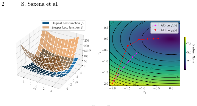
Theorem 1 is derived from standard assumptions without assuming its own conclusion. The proof bounds ||∇g_k||^2 and ∇f_k^T∇g_k using convexity and L-smoothness, then invokes the PL inequality to obtain linear convergence; no constant is fitted and the conclusion is not used as an input. The update in Eq. 9 is, by definition, gradient descent on g = f + λ||∇f||^2, so the theorem analyzes exactly the method it claims to analyze rather than a renamed version of the result. The illustrative f2 in Fig. 1 is explicitly constructed as the penalized f1, but the paper does not present the resulting trajectories as a derived prediction from the theorem. The equivalence with EGR is acknowledged in Section 5 ('Barrett and Dherin [1] proposed Explicit Gradient Regularization...'), so the 'new line-search method' framing is a novelty/attribution concern, not a circular derivation. The experimental comparisons are direct measurements; λ and α are chosen empirically, and the paper does not claim the theorem predicts the observed initial improvements. The lack of convergence proof for the CGD-FD/CGD-QN variants and the fallback branch is an incompleteness or overclaim issue, but it is not circularity because those parts are not derived from the theorem's assumptions and no fitted parameter is relabeled as a prediction.
Assumptions & free parameters
free parameters (4)
- λ (regularization coefficient) =
varies per function, e.g., 0.4, 0.5, 0.07, 10, 40, or L(0.01,0.1)
- α (step size) =
0.01 or 0.05 depending on function
- r (finite difference perturbation) =
not specified
- b (stopping threshold) =
T/4 = 10
assumptions (5)
- domain assumption f is twice differentiable on D
- domain assumption f is convex and L-smooth in Theorem 1
- domain assumption f satisfies the PL inequality for linear convergence
- standard math In the quadratic analysis, Q is symmetric positive definite and commutes with I
- ad hoc to paper The descent-direction check ∇f^T p_k < 0 is sufficient to guarantee that falling back to -∇f preserves convergence
Cite this review
Pith. "Pith review of CGD: Modifying the Loss Landscape by Gradient Regularization." pith.science (2026). https://pith.science/paper/RKTZMEQE
@misc{pith2026250416182,
  author       = {Pith},
  title        = {Pith review of: CGD: Modifying the Loss Landscape by Gradient Regularization},
  year         = {2026},
  howpublished = {\url{https://pith.science/paper/RKTZMEQE}},
  note         = {Machine review of arXiv:2504.16182}
}
read the original abstract
Line-search methods are commonly used to solve optimization problems. The simplest line search method is steepest descent where one always moves in the direction of the negative gradient. Newton's method on the other hand is a second-order method that uses the curvature information in the Hessian to pick the descent direction. In this work, we propose a new line-search method called Constrained Gradient Descent (CGD) that implicitly changes the landscape of the objective function for efficient optimization. CGD is formulated as a solution to the constrained version of the original problem where the constraint is on a function of the gradient. We optimize the corresponding Lagrangian function thereby favourably changing the landscape of the objective function. This results in a line search procedure where the Lagrangian penalty acts as a control over the descent direction and can therefore be used to iterate over points that have smaller gradient values, compared to iterates of vanilla steepest descent. We establish global linear convergence rates for CGD and provide numerical experiments on synthetic test functions to illustrate the performance of CGD. We also provide two practical variants of CGD, CGD-FD which is a Hessian free variant and CGD-QN, a quasi-Newton variant and demonstrate their effectiveness.
Figures


Figures from the paper (2 more)


Reference graph
Works this paper leans on
-
[1]
Barrett, D.G.T., Dherin, B.: Implicit gradient regularization (2022), https://arxiv. org/abs/2009.11162
arXiv 2022
-
[2]
Society for Industrial and Applied Mathematics (2014)
Beck, A.: Introduction to nonlinear optimization: Theory, algorithms, and appli- cations with MATLAB. Society for Industrial and Applied Mathematics (2014). https://doi.org/10.1137/1.9781611973655
-
[3]
Mathematics of Computation21(99), 368–381 (1967)
Broyden, C.G.: Quasi-newton methods and their application to function minimi- sation. Mathematics of Computation21(99), 368–381 (1967). https://doi.org/10. 1090/S0025-5718-1967-0224273-2 16 S. Saxena et al
work page 1967
-
[4]
Journal of Statistical Mechanics: Theory and Experiment2019(12), 124018 (2019)
Chaudhari, P., Choromanska, A., Soatto, S., LeCun, Y., Baldassi, C., Borgs, C., Chayes, J., Sagun, L., Zecchina, R.: Entropy-sgd: Biasing gradient descent into wide valleys. Journal of Statistical Mechanics: Theory and Experiment2019(12), 124018 (2019). https://doi.org/10.1088/1742-5468/ab39d9
-
[5]
In: Advances in Neural Information Processing Systems
Du, J., Zhou, D., Feng, J., Tan, V., Zhou, J.T.: Sharpness-aware train- ing for free. In: Advances in Neural Information Processing Systems. pp. 23439–23451 (2022), https://proceedings.neurips.cc/paper_files/paper/2022/file/ 948b1c9d660d7286dd767cd07dabd487-Paper-Conference.pdf
work page 2022
-
[6]
The Computer Journal 13(3), 317–322 (1970)
Fletcher, R.: A new approach to variable metric algorithms. The Computer Journal 13(3), 317–322 (1970). https://doi.org/10.1093/comjnl/13.3.317
-
[7]
Foret, P., Kleiner, A., Mobahi, H., Neyshabur, B.: Sharpness-aware minimization for efficiently improving generalization (2021), https://arxiv.org/abs/2010.01412
arXiv 2021
-
[8]
Neural Computation 9(1), 1–42 (1997)
Hochreiter, S., Schmidhuber, J.: Flat Minima. Neural Computation 9(1), 1–42 (1997). https://doi.org/10.1162/neco.1997.9.1.1
Show all 23 references
-
[9]
In: Proceedings of the 40th International Conference on Machine Learning
Karakida, R., Takase, T., Hayase, T., Osawa, K.: Understanding gradient regular- ization in deep learning: Efficient finite-difference computation and implicit bias. In: Proceedings of the 40th International Conference on Machine Learning. pp. 15809–15827 (2023), https://proce...
2023
-
[10]
In: Machine Learning and Knowledge Discovery in Databases
Karimi, H., Nutini, J., Schmidt, M.: Linear convergence of gradient and proximal- gradient methods under the polyak-łojasiewicz condition. In: Machine Learning and Knowledge Discovery in Databases. pp. 795–811 (2016). https://doi.org/10. 1007/978-3-319-46128-1_50
2016
-
[11]
Keskar, N.S., Mudigere, D., Nocedal, J., Smelyanskiy, M., Tang, P.T.P.: On large- batch training for deep learning: Generalization gap and sharp minima (2017), https://arxiv.org/abs/1609.04836
2017 arXiv
-
[12]
In: Advances in Neural Information Process- ing Systems (2018), https://proceedings.neurips.cc/paper_files/paper/2018/file/ a41b3bb3e6b050b6c9067c67f663b915-Paper.pdf
Li, H., Xu, Z., Taylor, G., Studer, C., Goldstein, T.: Visualizing the loss landscape of neural nets. In: Advances in Neural Information Process- ing Systems (2018), https://proceedings.neurips.cc/paper_files/paper/2018/file/ a41b3bb3e6b050b6c9067c67f663b915-Paper.pdf
2018
-
[13]
Springer New York, 2nd edn
Nocedal, J., Wright, S.J.: Numerical Optimization. Springer New York, 2nd edn. (2006). https://doi.org/10.1007/978-0-387-40065-5
2006 doi
-
[14]
Neural Computation 6(1), 147–160 (1994)
Pearlmutter, B.A.: Fast Exact Multiplication by the Hessian. Neural Computation 6(1), 147–160 (1994). https://doi.org/10.1162/neco.1994.6.1.147
1994 doi
-
[15]
USSR Com- putational Mathematics and Mathematical Physics 3(4), 864–878 (1963)
Polyak, B.: Gradient methods for the minimisation of functionals. USSR Com- putational Mathematics and Mathematical Physics 3(4), 864–878 (1963). https: //doi.org/10.1016/0041-5553(63)90382-3
1963 doi
-
[16]
J., P., Bodas, T.: Practical first-order bayesian optimization algorithms
Prakash, U., Chollera, A., Khatwani, K., K. J., P., Bodas, T.: Practical first-order bayesian optimization algorithms. In: Proceedings of the 7th Joint International Conference on Data Science & Management of Data (11th ACM IKDD CODS and 29th COMAD). p. 173–181 (2024). https:/...
2024
-
[17]
Ruder, S.: An overview of gradient descent optimization algorithms (2017), https: //arxiv.org/abs/1609.04747
2017 arXiv
-
[18]
In: Proceedings of the 32nd International Conference on Machine Learning
Schulman, J., Levine, S., Abbeel, P., Jordan, M., Moritz, P.: Trust region policy optimization. In: Proceedings of the 32nd International Conference on Machine Learning. pp. 1889–1897 (2015), https://proceedings.mlr.press/v37/schulman15. html
2015
-
[19]
Smith, S.L., Dherin, B., Barrett, D.G.T., De, S.: On the origin of implicit regular- ization in stochastic gradient descent (2021), https://arxiv.org/abs/2101.12176
2021 arXiv
-
[20]
Sutton, R.S., McAllester, D., Singh, S., Mansour, Y.: Policy gradient methods for reinforcement learning with function approximation. In: Advances in Neural In- CGD: Modifying the Loss Landscape by Gradient Regularization 17 formation Processing Systems (1999), https://proceed...
1999
-
[21]
Machine Learning8(3–4), 229–256 (1992)
Williams, R.J.: Simple statistical gradient-following algorithms for connectionist reinforcement learning. Machine Learning8(3–4), 229–256 (1992). https://doi.org/ 10.1007/bf00992696
1992 doi
-
[22]
In: Proceedings of the 39th International Confer- ence on Machine Learning
Zhao, Y., Zhang, H., Hu, X.: Penalizing gradient norm for efficiently improving generalization in deep learning. In: Proceedings of the 39th International Confer- ence on Machine Learning. pp. 26982–26992 (2022), https://proceedings.mlr.press/ v162/zhao22i.html
2022
-
[23]
Zhuang, J., Gong, B., Yuan, L., Cui, Y., Adam, H., Dvornek, N., Tatikonda, S., Duncan, J., Liu, T.: Surrogate gap minimization improves sharpness-aware training (2022), https://arxiv.org/abs/2203.08065
2022 arXiv
Reviewed August 16, 2026 · model on record in the stance chip above.
Discussion (0). Continue with ORCID to comment.