REVIEW 2 major objections 5 minor 20 references
Unexpected Effects of Online no-Substitution k-means Clustering
T0 review · 2 major / 5 minor · reviewed 2026-08-14 · deepseek-v4-flash
Pith's one-line read This paper proves the exact number of centers needed for constant-factor approximate online k-means: order and knowledge of n determine whether the answer is constant, logarithmic, or linear.
desk verdict The k-means characterization is real and the lower-bound machinery holds up, but the advertised universality for all triangle-type distances is false as stated; restrict Section 5's claim and the paper is solid. read the letter →
The pith
A machine-rendered reading of the paper's core claim, the machinery that carries it, and where it could break.
The reading
What carries the argument
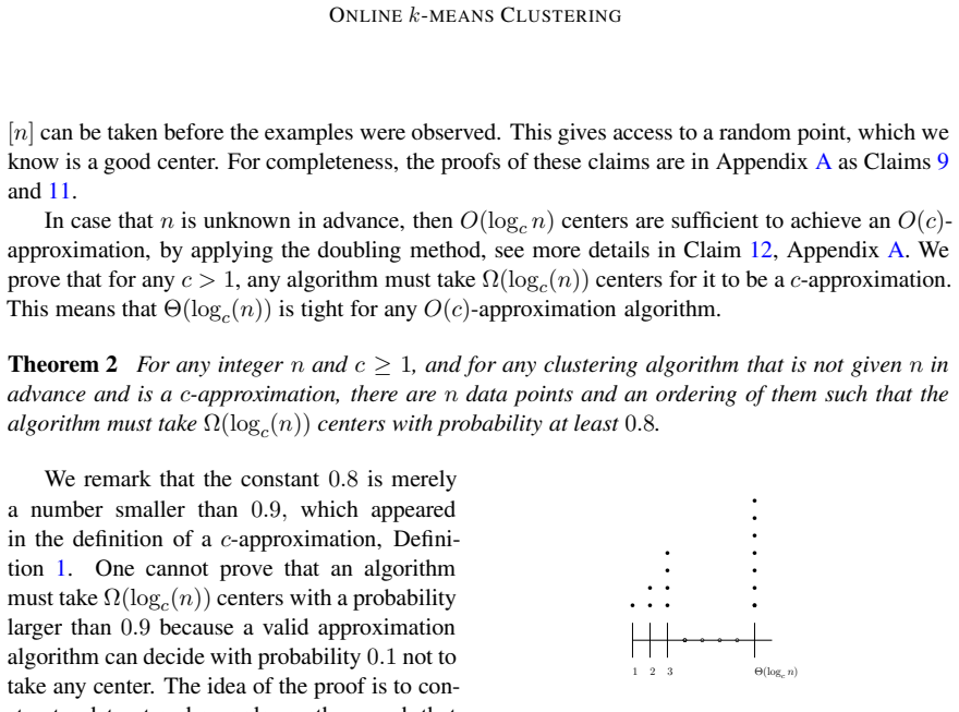
Two mechanisms carry the argument. The first is the random-point lemma: for squared Euclidean distance, $\mathbb{E}_{j}[\sum_i \|x_i-x_j\|^2] = 2\sum_i \|x_i-\mu\|^2$, so a uniformly random point in a cluster is a good center; this extends to any distance obeying $d(u,v) \le D(d(u,w)+d(w,v))$. The second is the layer-cake lower bound: an input of exponentially growing groups on the line, presented from smallest to largest, forces an algorithm that does not know $n$ to take a center from every group, because the stream may stop at any prefix. For the unknown-$n$ upper bound, the paper uses farthest-first traversal: the current point is taken as a center exactly when it is among the $k$ mutually farthest points seen so far, and this makes the $i$-th point a center with probability about $k/i$, yielding $O(k\log(n/k))$ centers.
What would settle it
Take the adversarial-order construction with $k=2$: choose $x_1=0$ and recursively choose $x_t$ so that $(x_t-x_{t-1})^2 > c\sum_{j<t}(x_{t-1}-x_j)^2$, then feed $x_1,\ldots,x_n$ in increasing order; any online no-substitution algorithm using $o(n)$ centers while keeping cost $\le c\cdot\operatorname{cost}(\mathrm{opt}_2)$ on every prefix with probability at least $0.9$ would refute the claimed $\Theta(n)$ lower bound. For the random-order unknown-$n$ case, simulate the same exponentially spaced values in uniformly random order and count how many record-farthest points must be taken; observing $o(\log n)$ centers for a $c$-approximation would refute the bound.
Extended reading notes
Core claim
The paper maps the full online no-substitution landscape for constant $k$. For $k=1$, one randomly chosen point is a constant-factor center when the order is random, and knowing $n$ lets a random index be chosen in advance; only with worst-case order and unknown $n$ does the requirement become $\Theta(\log n)$. For constant $k \ge 2$, the paper proves matching upper and lower bounds: $\Theta(n)$ centers under adversarial order, $\Theta(\log n)$ under random order with $n$ unknown, and $\Theta(1)$ under random order with $n$ known. The lower bounds use one-dimensional exponentially spaced constructions where every prefix could be the whole input, and the upper bounds are achieved by explicit algorithms: a three-phase wait-and-sample algorithm for known $n$, and a farthest-first-traversal rule for unknown $n$.
Load-bearing premise
The lower bounds for unknown $n$ assume the algorithm must be a $c$-approximation with probability at least $0.9$ on every possible input length, including every truncated prefix of the adversarial construction; if success were required only for the final known length, the $\Omega(\log n)$ lower bounds would not hold.
Editorial extensions
If this is right
- In the random-order, known-$n$ regime, an algorithm may deliberately observe a small random fraction of the data before choosing any center, and this waiting buys a constant number of centers.
- In the random-order, unknown-$n$ regime, no amount of cleverness can beat $\Theta(\log n)$ centers, so a simple farthest-first-traversal rule is optimal up to constants.
- Under adversarial order with $k \ge 2$, any algorithm that must succeed on every prefix must take essentially all points as centers, so useful guarantees require a weaker adversary or structural assumptions.
- Because the proofs only use a triangle-type inequality, the same center counts apply to $k$-medians and to $\ell_p$ costs with constant $p$, not just squared Euclidean distance.
- Dimension plays no role: the optimal bound in every regime is independent of the data's ambient dimension.
Reading between the lines
- Extension not made in the paper: if the success criterion were relaxed to require approximation only for the final, known stream length, the unknown-$n$ lower bounds would dissolve; one could test how the required center count interpolates between $\Theta(1)$ and $\Theta(\log n)$ when the algorithm is given only an upper bound on $n$.
- Extension not made in the paper: the unknown-$n$ upper bound stores all previous points to run farthest-first traversal, so it is not memory-efficient; a natural streaming extension would maintain an approximate farthest-first set and could be checked by simulation on random-order data.
- Extension not made in the paper: the same horizon-detection mechanism suggests that other single-pass decision problems with irreversible choices and unknown stream length will pay a logarithmic price, and the exponentially spaced line construction is a general template for proving such lower bounds.
Signed reviews
Editorial analysis
A structured set of objections, weighed in public.
Referee Report
Summary. The paper studies online no-substitution center-based clustering: points arrive one by one, and the algorithm must irrevocably decide whether to take the current point as a center. For k-means cost with a constant number k of clusters, it asks how many centers a constant-factor approximation requires, depending on whether the arrival order is random or adversarial and whether the dataset size n is known in advance. The main results are: (i) for k=1, Θ(1) centers are necessary and sufficient when the order is random or when n is known, and Θ(log n) when the order is adversarial and n is unknown; (ii) for constant k≥2, Θ(n) centers are necessary in adversarial order, Θ(1) centers with random order and known n, and Θ(log n) with random order and unknown n. The upper bounds are given by Algorithms 1, 2, 4 and a doubling method; the lower bounds are adversarial constructions over points on the line. The abstract and conclusion additionally claim that these bounds hold for any distance function satisfying a triangle-type inequality.
Significance. Restricted to Euclidean k-means, the paper is a solid and valuable contribution: it gives clean algorithmic ideas (sample-based thresholding in Algorithm 1, record-farthest selection in Algorithm 2, farthest-first traversal in Algorithm 4), states matching lower bounds, and the appendix contains explicit proofs. The unknown-n lower bounds are correctly interpreted as requiring success on every prefix, which is consistent with Definition 1 and is the standard meaning of not knowing n. However, the advertised universality over all D-costs is not merely unproved; it is false, and the counterexample is a valid metric satisfying Eq. (3). The Euclidean and ℓ_p results remain defensible after the generality claims are narrowed, but the current abstract and conclusion overstate the scope of the theorems.
major comments (2)
- [Abstract, §5, §6] The claim that the landscape in Figure 1 holds for every distance satisfying the triangle-type inequality (3) is not supported by Section 5 and is false. The lower-bound part of Section 5 explicitly needs extra structure: for k=1, Theorem 21 assumes points with d(x_i,x_j)=|j−i|, and for k≥2 the text requires a sequence with d(x_{i+1},x_i) ≥ c·d(x_i,x_{i−1}). Neither condition follows from (3). The discrete metric on n distinct points, d(x,y)=1 for x≠y, satisfies (3) with D=1, yet it has no such sequence for any c>1. In that metric any single center attains opt_1 exactly (both equal n−1) and any k distinct centers attain opt_k exactly for k≥2, so every cell of Figure 1 becomes Θ(1). This contradicts Theorem 2, Claim 13, and Theorem 4 if they are claimed to be universal. The universality sentence in the abstract and conclusion must be removed or qualified to the class of metrics that admit the line-like constructions used in the proofs.
- [§5, Theorem 21 and surrounding text] As a second consequence of the same gap, the general-cost k=1 lower bound is not proved for all D-costs. The text states, "assuming there are n points x_1,...,x_n with d(x_i,x_j)=|j−i|," and then Theorem 21 gives Ω(log n); Claim 22 supplies only the matching upper bound. Since such a line-embedded configuration may not exist in a given D-cost, the Θ(log n) entry for general costs is an upper bound without a corresponding lower bound. The proof of the k≥2 lower bound has the same structure, namely it needs a sequence whose consecutive distances grow by an arbitrary factor. The theorems should either be restricted to metrics that admit those sequences or the missing implication from (3) should be proved.
minor comments (5)
- [Theorem 2] Theorem 2 states "c ≥ 1", but the proof and the expression log_c n require c > 1; please restate the condition as c > 1.
- [§5, footnote 3] The footnote says d should "satisfy triangle inequality", while Eq. (3) is only a relaxed triangle inequality; the footnote should be aligned with Eq. (3).
- [Figure 1] The caption of Figure 1 is very compressed; the label "constant order" is ambiguous, and the reader must consult the text to determine which rectangle corresponds to adversarial order with unknown n.
- [Proof of Claim 18] In the proof of Claim 18 the record indicators are described as independent without justification; a one-sentence explanation (Rényi's argument for record indicators) would improve readability.
- [Algorithm 5] Algorithm 5 uses the variables "last" and "i*" before they are defined in the main text; moving the definitions before the pseudo-code would help the reader.
Circularity Check
No circularity: the central bounds are proved from explicit constructions and analyzed algorithms; the Section 5 universality overclaim is a correctness issue, not a circular derivation.
full rationale
The paper's central claims (the Θ(1), Θ(log n), and Θ(n) landscape in Figure 1) are derived from scratch. Upper bounds are given by explicit online algorithms (Algorithms 1, 2, 4, 5) and analyzed in Theorems 3, 5, 7 and Claims 12, 14, 15, 19, 20 using standard tools (a random point as a good center, Markov's inequality, random-sample concentration). Lower bounds are proved by explicit adversarial point series and prefix arguments: Theorem 2 uses exponentially repeated points on a line, Claim 13 and Theorem 4 use points with increasing distances so a furthest or k-maximal point must be taken before the stream may stop. No parameter is fitted to the quantity that is then called a prediction, and no theorem is imported from a self-citation as the load-bearing premise. The only self-citations (Bhattacharjee and Moshkovitz 2020; Hess et al. 2021) are explicitly presented as follow-up work and are not used to justify any bound. The manuscript itself flags a limitation in Section 5: the general-cost lower bounds require extra hypotheses, e.g., points with d(xi,xj)=|j−i| or consecutive distances growing by an arbitrary constant, and the abstract's unconditional 'any distance function that obeys a triangle-type inequality' is not established there and is false for a discrete metric. This is an overclaim or correctness defect, not a circular reduction: the Section 5 universality statement is not needed for the k-means-specific theorems, and the k-means results are independently proved. Hence the circularity score is 0.
Assumptions & free parameters
assumptions (5)
- domain assumption The distance function satisfies the D-relaxed triangle inequality (Inequality 3) for some constant D≥1.
- domain assumption The data points arrive in a uniformly random permutation when random order is assumed.
- standard math A constant-factor offline k-means approximation algorithm exists and is available as a subroutine.
- standard math Markov, Chebyshev, Hoeffding, and union-bound inequalities are used without proof.
- ad hoc to paper For every D-cost, there exists a series of points satisfying d(x_{i+1}, x_i) ≥ c·d(x_i, x_{i-1}) (or d(x_i,x_j)=|i-j|) to support the lower bounds.
Cite this review
Pith. "Pith review of Unexpected Effects of Online no-Substitution k-means Clustering." pith.science (2026). https://pith.science/paper/RLPBV63R
@misc{pith2026190806818,
  author       = {Pith},
  title        = {Pith review of: Unexpected Effects of Online no-Substitution k-means Clustering},
  year         = {2026},
  howpublished = {\url{https://pith.science/paper/RLPBV63R}},
  note         = {Machine review of arXiv:1908.06818}
}
read the original abstract
Offline k-means clustering was studied extensively, and algorithms with a constant approximation are available. However, online clustering is still uncharted. New factors come into play: the ordering of the dataset and whether the number of points, n, is known in advance or not. Their exact effects are unknown. In this paper we focus on the online setting where the decisions are irreversible: after a point arrives, the algorithm needs to decide whether to take the point as a center or not, and this decision is final. How many centers are needed and sufficient to achieve constant approximation in this setting? We show upper and lower bounds for all the different cases. These bounds are exactly the same up to a constant, thus achieving optimal bounds. For example, for k-means cost with constant k>1 and random order, Theta(log n) centers are enough to achieve a constant approximation, while the mere a priori knowledge of n reduces the number of centers to a constant. These bounds hold for any distance function that obeys a triangle-type inequality.
Figures

Figures from the paper (2 more)


Reference graph
Works this paper leans on
-
[1]
The number of centers the algorithm takes is Θ(1)
-
[2]
This is proved in Claims 14 and 15
cost(C) ≤ Θ(1) · cost(C ∗). This is proved in Claims 14 and 15. Claim 14 Algorithm 1 takes as center at most O(k5) points, with probability at least 0.98. Proof The algorithm takes as a center two types of points. Either cl ose (Line 19 in Algorithm 1) or far (Line 16). Bounding the number of close points by O(k2 log k) is easy, as it follows immediately ...
-
[3]
We cannot use this definition in our framework
Far points: in Indyk (1999), far points are the furthest points from the cluster defined in phase 1. We cannot use this definition in our framework. To resolve th is issue, we add an 22 ONLINE k-MEANS CLUSTERING intermediate step where the algorithm saves a constant frac tion of number of points to set a bar that defines far. In the last phase, only points t...
work page 1999
-
[5]
a point v ∈ C ∗ i will be taken as a center with ∑ x∈C∗ i d(x, v) ≤ 2D · cost(optk′)
-
[6]
cost(optk′−1) ≤ 13kD5a α · cost(optk′) Proof Focus on the closest point xi ∈ C ∗ i to the center c∗ i . The cost of taking xi as a center to C ∗ i is ∑ x∈C∗ i d(x, xi) ≤ D ∑ x∈C∗ i d(x, c∗ i ) + D ∑ x∈C∗ i d(c∗ i , xi) ≤ 2D ∑ x∈C∗ i d(x, c∗ i ), (7) in the first inequality we used Inequality 3 and in the second we used the fact that xi is closest to c∗ i t...
-
[7]
a point v ∈ C ∗ i will be taken as a center with that ∑ x∈C∗ i d(x, v) ≤ 5D2 · cost(optk′)
-
[8]
cost(optk′−1) ≤ 26kD5a α · cost(optk′) Proof Denote by Gi the |C∗ i | 2 closest points in C ∗ i to the center c∗ i . The cost of taking any g ∈ Gi as a center to C ∗ i is small ∑ x∈C∗ i d(x, g) ≤ D ∑ x∈C∗ i d(x, c∗ i ) + D ∑ x∈C∗ i d(g, c∗ i ) ≤ 5D2 ∑ x∈C∗ i d(x, c∗ i ), (8) where in the first inequality we used Inequality 3 and in the second we used the d...
work page 1999
-
[9]
If n is unknown in advance, one can use the doubling method. Claim 12 F or any c > 1 there is an algorithm that obtains O(c)-approximation with O(logc n) centers, no matter what the order is and even if n is unknown. Intuitively, since the algorithm does not know the value of n, it guess it and applies the algorithm from Theorem
Show all 20 references
-
[10]
In Indyk (1999), large means O(√n), as they cannot take more points for the algorithm to be with sublinear time
Parameter regime: “large” cluster in inherently differe nt in the two algorithms. In Indyk (1999), large means O(√n), as they cannot take more points for the algorithm to be with sublinear time. On the other hand, for Algorithm 1 “large” means some constant fraction because th...
1999
-
[11]
Once more data is arrived, it increases the value of n to c, and then to c2 and so on
The algorithm starts by assuming that n is small ( n = 1 ). Once more data is arrived, it increases the value of n to c, and then to c2 and so on. For each value of n, it applies the 15 ONLINE k-MEANS CLUSTERING algorithm from Theorem 11, i.e., picks one random point in the ne...
-
[12]
In our framework this is not allowed since once a center was ob served the algorithm cannot retake it
Centers from phase 1: Indyk (1999) simply takes the centers that were chosen in phase 1. In our framework this is not allowed since once a center was ob served the algorithm cannot retake it. To overcome this obstacle we take centers that are close to the centers chosen in pha...
1999
-
[13]
For any c-approximation it must take at least 0.5 of the maximal points with probability at least 0.8
-
[14]
Once we prove the two steps we are done
With probability at least 0.99 there are Ω(log n) maximal points. Once we prove the two steps we are done. Claim 1 - There are two cases (i) for each point if it’s a maxima l point, the probability the algorithm takes it as a center is at least 0.9 (ii) there is a point x that...
-
[15]
For any c-approximation it must take at least 0.5 of the k-maximal points with probability at least 0.8
-
[16]
The two claims follow from similar arguments as the proof of C laim 18
With probability at least 0.99 there are Ω( k log n k ) maximal points. The two claims follow from similar arguments as the proof of C laim 18. A.5.2. U PPER BOUNDS Proof [of Theorem 5] We start by bounding the number of expected centers the algo rithm uses. Denote by X the ra...
-
[17]
We know that |B| ≤ 0.01|C ∗ 2 | ≤ 0.02|Good2|
|B| ≤ 0.01|C ∗ 2 |: we will show that most probably, the first point the algorith m encounters in C ∗ 2 will be chosen as a center. We know that |B| ≤ 0.01|C ∗ 2 | ≤ 0.02|Good2|. Thus, with probability at least 1 − 0.02, the first point in Good2 ∪ B is in Good2 and the algorithm...
-
[18]
|B| > 0.01|C ∗ 2 |: we will show that C ∗ 1 and C ∗ 2 can be viewed as one cluster with x as its center without harming the cost by much. ∑ y∈C∗ 1 ∪C∗ 2 ‖y − x‖2 = ∑ y1∈C∗ 1 ‖y1 − x‖2 + ∑ y2∈C∗ 2 ‖y2 − x‖2 = ∑ y1∈C∗ 1 ‖y1 − x‖2 + ∑ y2∈C∗ 2 ‖(y∗ 2 − x) + (y2 − y∗ 2)‖2 ≤ ∑ y1∈C∗...
-
[19]
Number of centers is bounded by O(k log n k )
-
[20]
We prove the claim under the general cost function, see Section 5
cost(alg) ≤ Θ(1) · cost(optk) These claims are proved in Claims 19 and 20. We prove the claim under the general cost function, see Section 5. Claim 19 Algorithm 4 takes as center at most O(k log n k ), with probability at least 0.99. Proof To bound the number of centers the al...
2016
-
[21]
In Section B.2 we connect the optimal clustering and a clustering based on a random sample
In Section B.1 we analyze the expected appearance of a predetermined set in a random sample. In Section B.2 we connect the optimal clustering and a clustering based on a random sample. B.1. Random sample The next claim shows that for any predetermined set, with a hi gh probabi...
Reviewed August 14, 2026 · model on record in the stance chip above.
Discussion (0). Continue with ORCID to comment.