REVIEW 3 major objections 5 minor 31 references
Gaia Parallax of Milky Way Globular Clusters -- A Solution of Mixture Model
T0 review · 3 major / 5 minor · reviewed 2026-08-14 · deepseek-v4-flash
Pith's one-line read A two-component mixture model recovers the mean parallax of 120 globular clusters from Gaia DR2 parallaxes alone, sidestepping cluster membership determination entirely.
desk verdict Useful membership-free GC parallax catalog, but the field-profile assumption needs stronger validation. read the letter →
The pith
A machine-rendered reading of the paper's core claim, the machinery that carries it, and where it could break.
The reading
What carries the argument
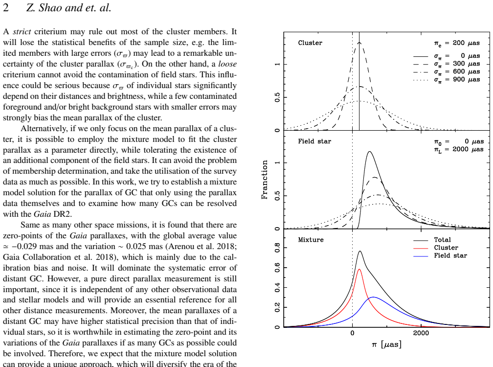
The central object is the two-component parallax mixture model. The cluster component is a delta function at the mean parallax $\varpi_c$; the field component follows the exponentially decreasing density profile of Bailer-Jones et al. (2018), $\varphi_f(\varpi)=\frac{\varpi_L^3}{2(\varpi-\varpi_0)^4}\exp\left(-\frac{\varpi_L}{\varpi-\varpi_0}\right)$ for $\varpi>\varpi_0$. Each component is convolved with the per-star Gaussian parallax error, and the model is fitted by nested sampling, with $\varpi_c$ obtained by marginalizing over $\varpi_0$, $\varpi_L$, and the cluster fraction $n_c$. The asymmetry of the field profile is what lets the model peel a symmetric cluster signal out of a heavily contaminated, error-dominated parallax histogram.
What would settle it
Fit the mixture model to synthetic sight lines drawn from a realistic Galactic model whose field-star parallax distribution is not exponential (e.g., including bulge and spiral-arm structure) over the same distance and contamination ranges as the Pancino et al. (2017) simulations; if the recovered $\varpi_c$ deviates from the input by more than the 1-5% claimed accuracy, the exponential field profile is the cause. Alternatively, test a real line of sight where a known foreground structure creates a secondary bump in the parallax histogram and check whether the mixture model misattributes it to the cluster.
Extended reading notes
Core claim
The central claim is that a mixture model fitted to raw parallax histograms alone can separate a cluster's mean parallax $\varpi_c$ from field-star contamination without membership determination. The cluster is modeled as a delta function at $\varpi_c$, the field by the skewed exponentially decreasing density profile of Bailer-Jones et al. (2018), and each is convolved with per-star Gaussian errors. Nested sampling fits the four parameters and then marginalizes out the field parameters to obtain a posterior for $\varpi_c$. On the 18 simulated clusters of Pancino et al. (2017) the recovered $\varpi_c$ matches the input and remains stable when the fitted aperture is varied. Applied to Gaia DR2, 120 globular clusters are resolved, and comparison with indirect distances gives an offset of $-27.6\pm1.7\,\mu\mathrm{as}$ and a scatter of $22.8\pm1.3\,\mu\mathrm{as}$, consistent with the known Gaia DR2 zero-point and its variation.
Load-bearing premise
The separation of cluster from field rests on the assumed analytic form of the field-star parallax distribution (Eq. 3, a simple exponentially decreasing density profile); if the true field in a cluster direction is more complex, the fitted cluster parallax can absorb the model mismatch and become biased.
Editorial extensions
If this is right
- The mixture model can be applied to future Gaia data releases with no membership determination, so the direct-parallax sample of globular clusters will grow as astrometric precision improves.
- The 120 resolved clusters constitute the largest set of independent direct parallaxes, providing tracers for monitoring the Gaia zero-point and its spatial variation.
- For the nearest clusters such as M 4 and NGC 6397, the statistical precision reaches a fraction of a percent, comparable to or better than many indirect distance methods.
- In heavily contaminated fields like M 62, the mixture model avoids the bias that membership-based direct measurements can suffer, because it does not need to discard field stars.
- The measured offset of about $-27.6\,\mu\mathrm{as}$ between apparent mixture-model parallaxes and indirect distances independently confirms the global Gaia DR2 zero-point.
Reading between the lines
- If the field-star model were replaced by a more realistic multi-component Galactic model (disc, bulge, halo), the method could likely resolve more of the 27 rejected clusters and reduce the scatter in the zero-point comparison.
- The same mixture approach could be applied to open clusters, dwarf spheroidal galaxies, or any compact stellar system whose mean parallax is contaminated by foreground and background stars in Gaia-like catalogs.
- Because the authors caution that the fitted $\varpi_0$ is only nominal, a natural extension is to calibrate the field profile against quasar-based zero-point maps and turn the apparent cluster parallaxes into absolute distances with per-cluster corrections.
- The significant disagreements with H18 for NGC 6397, $\omega$ Cen, and M 62 indicate method-dependent biases; a combined analysis using colour-magnitude-based membership posteriors would show whether the mixture model or the membership approach is wrong in those fields.
Signed reviews
Editorial analysis
A structured set of objections, weighed in public.
Referee Report
Summary. The paper proposes a two-component mixture model to derive the mean parallax of Milky Way globular clusters directly from Gaia DR2 parallaxes, thereby avoiding explicit membership determination: the cluster term is a delta function convolved with the per-star parallax errors, and the field term follows the exponentially decreasing density profile of Bailer-Jones et al. (2018), Eq. (3). The model is validated on the 18 simulated clusters of Pancino et al. (2017), applied to 147 clusters from Kharchenko et al. (2013), and 120 are reported as successfully resolved. The fitted apparent parallaxes are compared with the direct parallaxes of Gaia Collaboration et al. (2018) and with indirect distance catalogs; a combined offset of -27.6 +/- 1.7 microarcseconds and scatter of 22.8 +/- 1.3 microarcseconds are interpreted as a confirmation of the known Gaia DR2 parallax zero-point and its variation. The paper also discusses distances of five nearby clusters after applying a -29 microarcsecond zero-point correction.
Significance. If the central claim is correct, this is a genuinely useful contribution: it provides the largest direct-parallax catalog of Milky Way globular clusters and offers an independent route that does not depend on proper-motion or CMD membership selection. The likelihood, nested-sampling implementation, marginalization over nuisance parameters, and validation on the P17 simulated clusters are clearly described, and the authors are honest that the fitted zero-point parameter is only nominal and cannot be used directly for the Gaia zero-point. The comparison with independent catalogs is appropriate for a first demonstration, and the claimed offset is consistent with the known Gaia DR2 zero-point. The main limitation is that the robustness of the recovered cluster parallax against misspecification of the field-star parallax distribution is not established for real Milky Way fields, which is exactly the regime where the method is intended to be used.
major comments (3)
- [Sec. 2.2, Eq. (3)] The load-bearing assumption is that any mismatch between the true field-star parallax distribution and the simple exponentially decreasing profile of Eq. (3) is absorbed by the nuisance parameters n_c, omega_L, and omega_0, rather than leaking into the cluster parallax omega_c. The paper itself notes that omega_0 shifts to compensate for model mismatch, but the claim that omega_c is unaffected is demonstrated only on the 18 P17 simulated clusters, each of which has a single background component (halo, disc, or bulge). Real fields, especially toward the bulge, can contain multiple overlapping stellar populations and extinction structure, and the cluster term - a symmetric Gaussian whose width is tied to the per-star sigma_pi - is the only remaining flexible symmetric component that can absorb an asymmetric field residual. I recommend adding a quantitative test in which synthetic cluster populations with known parallax and known n_c are injected into real Gaia DR2 field-star samples (e.g., from annuli around clusters or from adjacent control fields) and the recovery of omega_c is checked as a function of field complexity. Without such a test, the validity of the 120-cluster catalog and of the -27.6 +/- 1.7 microarcsecond zero-point offset is not fully established for realistic fields.
- [Sec. 3, radius selection and cluster rejection] The construction of the final catalog involves data-dependent selection choices that are not covered by the P17 simulation validation. The fitting radius is chosen from r1, (r0+r1)/2, or r0 based on the overdensity and the stability of the fits, and 27 of 147 clusters are rejected because the marginal PDF of omega_c is not single-mode or because the result is not stable over a range of radii. Because both the radius choice and the acceptance criterion are made after inspecting the same data, there is a risk of selection bias: clusters with problematic fields may be preferentially excluded, while the reported scatter and offset are computed on the accepted sample. I ask the authors to report, for every cluster, which radius was used and why, to quote the number of clusters that failed at each selection stage, and to show for all 120 accepted clusters that varying the radius within the stated range changes omega_c by less than the statistical error. It would also be useful to test whether acceptance or rejection correlates with position on the sky, distance, or field density, since such a correlation would indicate that the field model, not the cluster signal, is driving the selection.
- [Sec. 4.1, comparison with H18] The comparison with the H18 membership-based parallaxes shows that 9 of 75 clusters (12%) exceed the 2-sigma combined uncertainty and 5 exceed 3-sigma. The authors attribute part of this to contamination in the H18 membership sample and discuss M 62 as a specific case. However, the opposite failure mode is never tested: a cluster component created by unmodeled field structure could produce a spurious omega_c, and because the method uses no membership information, this possibility cannot be excluded a priori. The M 62 discussion shows that membership contamination can be severe, but it does not establish that the mixture model cannot produce a false positive in dense bulge fields. I recommend testing for false positives by applying the mixture model to control fields with no known cluster, or by injecting synthetic clusters of known parallax and measuring the rate of spurious detection as a function of field density. Without this test, the 12% discrepant fraction is more naturally read as evidence that at least one of the two methods is biased in a nontrivial subset of fields, and the direction of the bias is not determined by the comparison presented.
minor comments (5)
- [Sec. 2.2, Eq. (8)] The text refers to the 'joint logistical likelihood'; this should read 'joint log-likelihood' or 'logarithmic likelihood'.
- [Sec. 2.2 and Fig. 4] The sentence 'Fitting results are plotted in figure 1' appears to refer to the 18-simulated-cluster comparison shown in Figure 4; the cross-reference should be corrected.
- [Sec. 3] The outlier cut 'omega + 0.029 mas < -3 sigma_pi' is dimensionally confusing as written; please restate with explicit units, e.g., 'omega/arcsec + 0.000029 < -3 sigma_pi'.
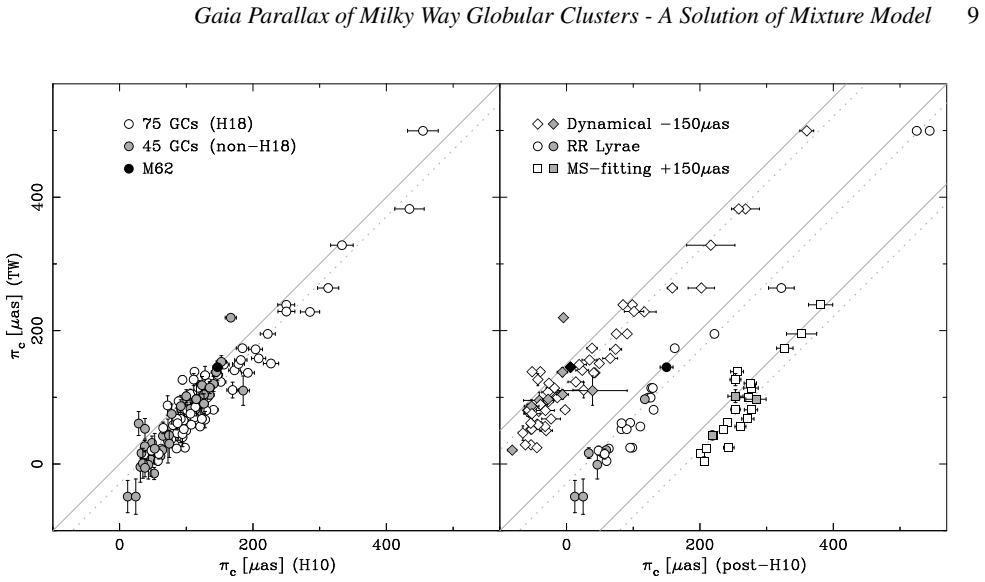
- [Sec. 4.2] When converting H10 distance moduli to parallaxes, the paper states that a 0.1 mag error is assumed for all clusters, but it does not describe how this error is propagated to the parallax comparisons; please specify the conversion and the treatment of asymmetric distance errors.
- [Abstract] The phrase 'They construct the largest direct parallax sample up to now' is awkward because the antecedent is unclear; consider 'This sample constitutes the largest direct-parallax catalog of globular clusters to date.'
Circularity Check
No significant circularity: the cluster parallax is a fitted parameter of an explicit mixture model, validated on external simulations and compared with independent measurements after the fit.
full rationale
The paper's central output, the cluster parallax ϖc, is an explicit free parameter of a likelihood built from an assumed mixture of a delta-function cluster component (Eq. 2) and a field component (Eq. 3), with individual errors convolved as Gaussians (Eqs. 4–8). The value is estimated by Nested Sampling from the Gaia parallax data themselves; it is not defined in terms of, or constrained by, the indirect distances, the H18 results, or the Gaia zero-point discussed later. Validation is external: 18 simulated clusters of Pancino et al. (2017) with known input parallaxes are recovered, and the recovered values are compared with the true inputs, not with the model outputs. The comparisons with H18 direct parallaxes and with indirect distances (H10, post-H10) are performed after fitting, and the resulting offset (−27.6 ± 1.7 μas) is reported as a measurement consistent with the known Gaia zero-point; that zero-point is not inserted into the model to force the result. There are no load-bearing self-citations, no uniqueness theorem imported from the authors' prior work, and no fitted quantity is renamed as a prediction. The acknowledged modeling limitation—that Eq. (3) is an approximation and the fitted ϖ0 is only nominal—raises a genuine identifiability risk that field-model misspecification could bias ϖc, but that is a statistical robustness concern explicitly flagged by the authors, not a circular reduction of the derivation to its inputs. The derivation chain is therefore self-contained and non-circular.
Assumptions & free parameters
free parameters (5)
- Cluster parallax omega_c =
fitted per cluster; example 499.5 microarcseconds for M4
- Cluster fraction n_c =
fitted per cluster
- Field scale parameter omega_L =
fitted per cluster
- Field zero-point parameter omega_0 =
fitted per cluster
- Fitting radius choice =
chosen per cluster from r1, (r0+r1)/2, r0
assumptions (6)
- domain assumption The intrinsic cluster parallax distribution is a delta function (Eq. 2).
- domain assumption Field-star parallaxes follow the exponentially decreasing density profile of Eq. (3) (Bailer-Jones et al. 2018).
- domain assumption Gaia DR2 parallax uncertainties are Gaussian and known after scaling by 1.081 (Lindegren et al. 2018).
- standard math The joint likelihood is a product of independent mixture densities and Nested Sampling yields valid marginal posteriors.
- domain assumption Radial and magnitude-dependent incompleteness changes only the cluster fraction n_c, not the fitted omega_c.
- domain assumption The cluster centers and characteristic radii from Kharchenko et al. (2013) are accurate.
Cite this review
Pith. "Pith review of Gaia Parallax of Milky Way Globular Clusters -- A Solution of Mixture Model." pith.science (2026). https://pith.science/paper/RP3EDNSO
@misc{pith2026190806031,
  author       = {Pith},
  title        = {Pith review of: Gaia Parallax of Milky Way Globular Clusters -- A Solution of Mixture Model},
  year         = {2026},
  howpublished = {\url{https://pith.science/paper/RP3EDNSO}},
  note         = {Machine review of arXiv:1908.06031}
}
abstract
We have established a mixture model approach to derive the parallax of the Milky Way globular clusters. It avoids the problem of cluster membership determination and provides a completely independent astrometrical solution by purely using the parallax data. This method is validated with simulated clusters of \cite{2017MNRAS.467..412P}. We have resolved 120 real globular clusters by the mixture model using parallaxes of the second data release of \gaia. They construct the largest direct parallax sample up to now. In comparing with other direct parallax results based on cluster members, including 75 clusters of \cite{2018A&A...616A..12G}, our method presents its accuracy, especially for some particular clusters. A systematic offset of $-27.6\pm1.7$ $\mu$as, together with a scatter of $22.8\pm1.3$ $\mu$as is found in comparing with other indirect parallax measurements. They are consistent with the global value and the variation of the zero-point of current \gaia parallaxes. Distances of several specific nearby globular clusters are discussed while the closest ones can reach high precisions, even taking the systematic error into account.
Figures


Figures from the paper (4 more)


Reference graph
Works this paper leans on
-
[1]
Arellano Ferro A., Ahumada J. A., Bustos Fierro I. H., Calder \'o n J. H., Morrell N. I., 2018, AN, 339, 183
work page 2018
-
[2]
Arenou F., et al., 2018, A&A, 616, A17
work page 2018
-
[3]
Bailer-Jones C. A. L., Rybizki J., Fouesneau M., Mantelet G., Andrae R., 2018, AJ, 156, 58
work page 2018
-
[4]
Baumgardt H., Hilker M., 2018, MNRAS, 478, 1520
work page 2018
- [5]
-
[6]
M., Casertano S., Strader J., Riess A., VandenBerg D
Brown T. M., Casertano S., Strader J., Riess A., VandenBerg D. A., Soderblom D. R., Kalirai J., Salinas R., 2018, ApJ, 856, L6
work page 2018
-
[7]
G., Recio-Blanco A., Lucatello S., D'Orazi V., Cassisi S., 2010, A&A, 516, A55
Carretta E., Bragaglia A., Gratton R. G., Recio-Blanco A., Lucatello S., D'Orazi V., Cassisi S., 2010, A&A, 516, A55
work page 2010
-
[8]
Chen S., Richer H., Caiazzo I., Heyl J., 2018, ApJ, 867, 132
work page 2018
Show all 31 references
-
[9]
A., Pritzl B
Contreras R., Catelan M., Smith H. A., Pritzl B. J., Borissova J., Kuehn C. A., 2010, AJ, 140, 1766
2010
-
[10]
P., Cameron E., Pettitt A
Feroz F., Hobson M. P., Cameron E., Pettitt A. N., 2013, arXiv:1306.2144
2013 arXiv
-
[11]
Gaia Collaboration, et al., 2018, A&A, 616, A1
2018
-
[12]
Gaia Collaboration, et al., 2018, A&A, 616, A12 (H18)
2018
-
[13]
Gaia Collaboration, et al., 2016, A&A, 595, A1
2016
-
[14]
E., 1996, AJ, 112, 1487 (H10)
Harris W. E., 1996, AJ, 112, 1487 (H10)
1996
-
[15]
Hernitschek N., et al., 2019, ApJ, 871, 49
2019
-
[16]
Kaluzny J., et al., 2013, AJ, 145, 43
2013
-
[17]
V., Piskunov A
Kharchenko N. V., Piskunov A. E., Schilbach E., R \"o ser S., Scholz R.-D., 2012, A&A, 543, A156
2012
-
[18]
V., Piskunov A
Kharchenko N. V., Piskunov A. E., Schilbach E., R \"o ser S., Scholz R.-D., 2013, A&A, 558, A53
2013
- [19]
-
[20]
L., Walker A., 2014, ApJS, 210, 6
Lee J.-W., L \'o pez-Morales M., Hong K., Kang Y.-W., Pohl B. L., Walker A., 2014, ApJS, 210, 6
2014
-
[21]
Lindegren L., et al., 2018, A&A, 616, A2
2018
-
[22]
R., et al., 2015, ApJ, 808, 11
Neeley J. R., et al., 2015, ApJ, 808, 11
2015
-
[23]
M., Gilligan C., Chaboyer B., 2017, ApJ, 838, 162
O'Malley E. M., Gilligan C., Chaboyer B., 2017, ApJ, 838, 162
2017
-
[24]
Pancino E., Bellazzini M., Giuffrida G., Marinoni S., 2017, MNRAS, 467, 412 (P17)
2017
-
[25]
Randich S., et al., 2018, A&A, 612, A99
2018
-
[26]
F., Cudworth K
Rees R. F., Cudworth K. M., 2017, AAS, 229, 343.07
2017
-
[27]
A., Denissenkov P
VandenBerg D. A., Denissenkov P. A., 2018, ApJ, 862, 72
2018
-
[28]
A., Denissenkov P
VandenBerg D. A., Denissenkov P. A., Catelan M., 2016, ApJ, 827, 2
2016
-
[29]
L., van der Marel R
Watkins L. L., van der Marel R. P., 2017, ApJ, 839, 89
2017
-
[30]
L., van der Marel R
Watkins L. L., van der Marel R. P., Bellini A., Anderson J., 2015, ApJ, 812, 149
2015
-
[31]
A., et al., 2012, AJ, 143, 50
Woodley K. A., et al., 2012, AJ, 143, 50
2012
Reviewed August 14, 2026 · model on record in the stance chip above.
Discussion (0). Continue with ORCID to comment.