Pith. sign in

REVIEW 3 minor 37 references

A tutorial reviews fundamental physical bounds on light-matter interactions across scales in photonics and electromagnetics.

Reviewed by Pith at T0; open to challenge. T0 means a machine referee read the full paper against a public rubric. the ladder, T0–T4 →

A tutorial that reviews and unifies prior results on fundamental limits of optical material responses, wave propagation, scattering, and related phenomena.

T0 review reviewed 2026-06-30 challenge →

load-bearing objection This is a tutorial review that organizes existing bounds on light-matter interactions but introduces no new results or frameworks.

arxiv 2605.24738 v1 pith:RQBQOHZX submitted 2026-05-23 physics.optics

Fundamental limits in photonics and electromagnetics: a tutorial

classification physics.optics
keywords fundamental limitsphotonicselectromagneticslight-matter interactionsphysical boundswave propagationscatteringtutorial
verification ladder T0 review T1 audit T2 compute T3 formal T4 reserved

The pith

A machine-rendered reading of the paper's core claim, the machinery that carries it, and where it could break.

The reading

The paper reviews the fundamental principles constraining light-matter interactions and organizes limits by hierarchical scale, from optical material responses through wave propagation and scattering to functional phenomena. It aims to unify prior results on these bounds while identifying open questions that remain in the field. This synthesis is intended to let readers quickly engage with the current frontier and help build toward a universal framework for light interactions with matter.

Core claim

The tutorial synthesizes existing physical bounds and constraints on light-matter interactions, structured hierarchically from material responses to wave propagation, scattering, and related optical functions, while highlighting unresolved questions to support progress on a universal framework.

What carries the argument

Hierarchical scales of limits, from optical material responses to wave propagation, scattering, and optical phenomena and functions.

Load-bearing premise

The tutorial's selection and synthesis of prior literature accurately and comprehensively represents the key limits without significant omissions or interpretive bias.

What would settle it

Discovery of a major physical bound or constraint in photonics or electromagnetics that is omitted from the tutorial or presented with clear interpretive error.

Watch this falsifier. Get emailed when new claim-graph text bears on it.

Share X Bluesky LinkedIn Reddit HN

Editorial analysis

A structured set of objections, weighed in public.

Desk editor's note, referee report, simulated authors' rebuttal, and a circularity audit.

Referee Report

0 major / 3 minor

Summary. The manuscript is a tutorial review that first outlines fundamental principles constraining light-matter interactions in photonics and electromagnetics, then surveys physical bounds and limits across hierarchical scales (optical material responses, wave propagation, scattering, and related functions), and concludes by advocating a unified treatment while identifying open questions to accelerate reader entry into the research frontier.

Significance. If the synthesis accurately and comprehensively represents the cited literature without interpretive bias, the tutorial would provide a useful entry point for newcomers by consolidating disparate bounds into one narrative and flagging unresolved issues; the absence of new derivations or predictions means its value rests entirely on the quality of the literature selection and organization.

minor comments (3)
  1. The abstract states the goal of a 'more unified treatment,' but the manuscript should explicitly define what unification means (e.g., common mathematical framework, shared assumptions across scales) in an early section to avoid the impression of a simple juxtaposition of results.
  2. Several cited limits (e.g., those derived from causality or passivity) are referenced without a brief recap of their key assumptions or the precise statement of the bound; adding one-sentence reminders would improve accessibility for readers new to the sub-area.
  3. The discussion of open questions at the end would benefit from a short table or enumerated list that cross-references each question to the relevant earlier section, making the connection between reviewed results and frontiers more concrete.

Simulated Author's Rebuttal

0 responses · 0 unresolved

We thank the referee for their positive summary of the manuscript and for recommending minor revision. The report correctly identifies the tutorial's scope and intent to consolidate bounds across scales while highlighting open questions. No specific major comments were raised.

Circularity Check

0 steps flagged

No circularity: tutorial synthesis of external literature

full rationale

The paper is explicitly a tutorial review whose purpose is to synthesize and unify existing results on physical bounds in photonics and electromagnetics drawn from prior literature. No original derivations, quantitative predictions, fitted parameters, or new technical claims are advanced that could reduce by construction to self-citations or inputs. The abstract and structure confirm the work reviews fundamental principles at multiple scales and highlights open questions without introducing load-bearing steps that equate to the paper's own content. As a result the derivation chain is absent and the content remains self-contained against external benchmarks.

Axiom & Free-Parameter Ledger

0 free parameters · 0 axioms · 0 invented entities

As a tutorial review, the paper introduces no new free parameters, axioms, or invented entities; it relies on standard principles from prior physics literature.

reviewed 2026-06-30 · how reviews work

0 comments
Cite this review

Pith. "Pith review of Fundamental limits in photonics and electromagnetics: a tutorial." pith.science (2026). https://pith.science/paper/RQBQOHZX

@misc{pith2026260524738,
  author       = {Pith},
  title        = {Pith review of: Fundamental limits in photonics and electromagnetics: a tutorial},
  year         = {2026},
  howpublished = {\url{https://pith.science/paper/RQBQOHZX}},
  note         = {Machine review of arXiv:2605.24738}
}
Share X Bluesky LinkedIn Reddit HN
read the original abstract

Theoretical limits and physical bounds across many areas of science, mathematics, and technology -- including Shannon's information-capacity limits, Bennett and Landauer's thermodynamic limits on computation, and G\"odel's incompleteness theorem in formal logic -- serve as defining pillars of their fields. In photonics and electromagnetism, numerous physical bounds and constraints have likewise been uncovered over the past several decades. In this Tutorial, we first review the fundamental principles that constrain light-matter interactions, and then discuss limits at different hierarchical scales, from optical material responses to wave propagation, scattering, and related optical phenomena and functions, relevant to a wide range of applications. By providing a more unified treatment of these results and highlighting the many open questions that remain, our goal is to help readers rapidly get up to speed with the frontier of this research area and contribute to advancing the broader vision of a universal framework for fundamental limits of light interactions with matter.

Figures

Figures reproduced from arXiv: 2605.24738 by Francesco Monticone, Owen D. Miller.

Figure 1
Figure 1. Figure 1: Overview of the manuscript, illustrating the fundamental principles and broad classes of bounds discussed in this Tutorial. A brief sixth chapter looks forward [PITH_FULL_IMAGE:figures/full_fig_p006_1.png] view at source ↗
Figure 2
Figure 2. Figure 2: Causality, absorption, and frequency dispersion. Thought experiment illus￾trating the fundamental connection between causality and dispersion. An input signal that is zero for t < 0 can be expressed as a superposition of harmonic components, each of which individually extends from t = −∞ to t = +∞. A system that absorbs only a single frequency component while leaving all others unaffected would necessarily… view at source ↗
Figure 3
Figure 3. Figure 3: Maximum refractive index. (a) Schematic of a single Drude–Lorentz oscillator illustrating the tradeoff between refractive index and dispersion. Lowering the resonance frequency ω0 increases the ratio ω 2 p/ω 2 0 , thereby enhancing the maximum refractive index nmax at frequency ω, but at the expense of increased dispersion dn/dω. The plasma frequency ωp = p Ne2/(ε0me) and, hence, the oscillator strength, a… view at source ↗
Figure 4
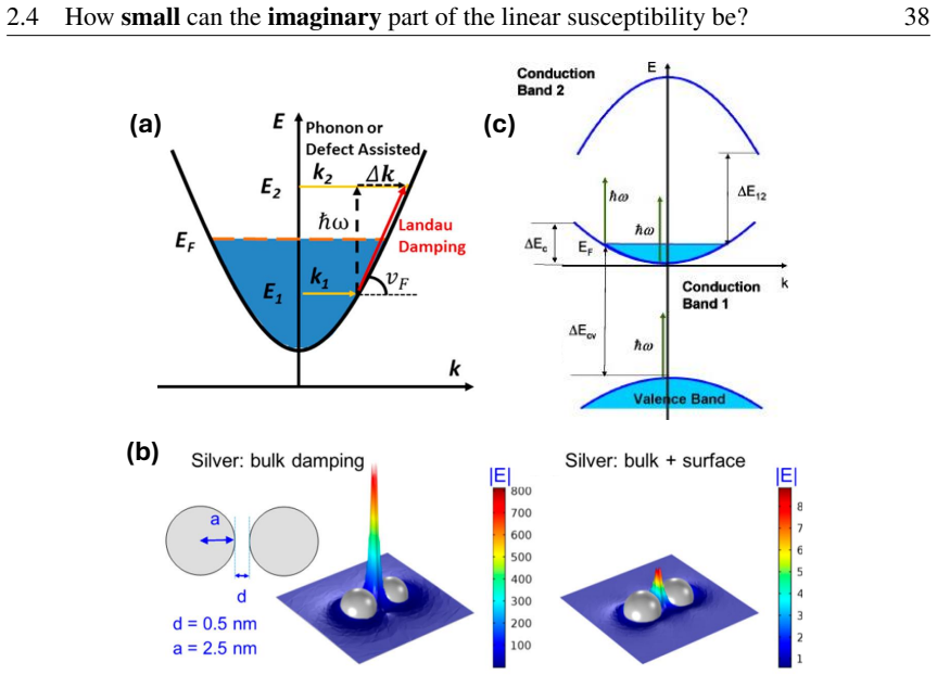
Figure 4. Figure 4: Lossy and lossless metals. (a) Absorption in metals: Absorption of a photon with small momentum/wavevector assisted by a phonon or defect (dashed arrows), or direct ab￾sorption of a confined surface plasmon-polariton (SPP) with large momentum/wavevector (solid arrow), corresponding to Landau damping (surface-collision assisted damping). (b) Example illustrating the impact of Landau damping: SPP field distr… view at source ↗
Figure 5
Figure 5. Figure 5: Bounds on resonant nonlinear susceptibilities. (a) Schematic of a three￾level system used for a second-order sum-frequency generation (SFG) process (left), together with the corresponding physical bound on the normalized oscillator strength of the doubly resonant second-order susceptibility, χ (2) , as a function of photon energy. The plot compares the physical bound with experimental measurements (black d… view at source ↗
Figure 6
Figure 6. Figure 6: Mechanisms and energy requirements for large refractive-index modulation. (a) Schematic of a typical anharmonic potential U(x) of depth U0. The refractive index depends on its local curvature, averaged over all electrons, ⟨d 2U(x)/dx2 ⟩N, and on the electron density N [122]. (b) The overall curvature can be changed through lattice distortion induced by temperature, strain, or an applied electric field (or … view at source ↗
Figure 7
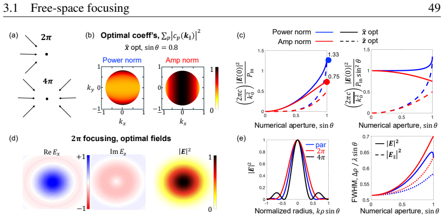
Figure 7. Figure 7: Plane-wave focusing. (a) Schematic of the 2π and 4π aperture limits. (b) Optimal focusing coefficients, as a function of wavenumbers kx and ky, for sinθ = 0.8. When normalizing by amplitude, the smaller kx values have the largest relative contribution to |Ex| 2 ; when normalizing by power, the large-kx waves have cancelling transverse power flows and hence are the coefficients to maximize. (c) Maximum valu… view at source ↗
Figure 8
Figure 8. Figure 8: Comparison of optimal focusing fields. Radial fields in the paraxial, 2π, and 4π apertures. One can see that maximally intense fields broaden a bit as their numerical aperture increases from paraxial to 2π, but then significantly tighten in going from 2π to 4π, with a corresponding intensity increase in the 4π limit. A comparison with the paraxial Eq. (91) and 2π Eq. (92) distributions is shown in [PITH_F… view at source ↗
Figure 9
Figure 9. Figure 9: Bounds on focal-point intensity subject to a spot-size constraint. (a) Optimal radial intensity profiles, in the paraxial limit, for normalized zero-field spot sizes ranging from G = 0.5λ down to 0.1λ. (b) Maximal Strehl ratio Smax as a function of G, exhibiting the universal G 4 scaling at small G. Markers indicate previously proposed designs, which fall well below the bound at moderate G (see Ref. [148] … view at source ↗
Figure 10
Figure 10. Figure 10: Space-time-optimal focusing (1D). Left: The full electric field E(x,t), with two counter-propagating wave packets along x = ±ct coherently summing to a sharp focus at the spacetime origin; the dotted line marks the t = 0 cross-section. Right: The spacetime-focused field E(x,0) (blue) is broader than its single-frequency counterpart (orange), due to the collective contributions of smaller frequencies which… view at source ↗
Figure 11
Figure 11. Figure 11: Partial time reversal at an outer boundary. Four-step construction underlying Eq. (113). (1) The interior sources s0 (purple, possibly within scatterers shown in grey) radiate fields ψ under outgoing boundary conditions (PML). (2) “Perfectly cancelling cur￾rents” spcc are added on an exterior surface (dashed) via the surface-equivalence principle, exactly nulling the field outside; the now-zero exterior a… view at source ↗
Figure 12
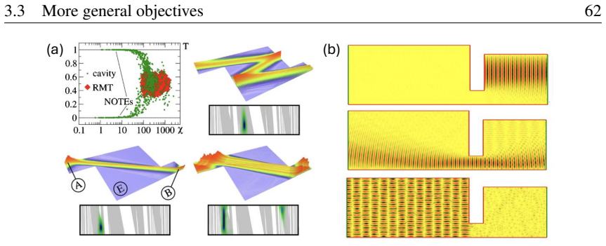
Figure 12. Figure 12: Wigner–Smith time-delay extremal modes. (a) Examples of wave functions that minimize time delay between ports/leads for a strongly scattering rectangular cavity. These modes (termed “NOTEs”) show quite different transmission statistics than those predicted by random matrix theory (RMT), and allow the possibility for a sender (“A”) to transmit to a receiver (“B”) while circumventing an eavesdropper (“E”). … view at source ↗
Figure 13
Figure 13. Figure 13: A powerful method for complete coupling of free-space waves to guided modes. (a) Maximally focusing the incident field (including reflections from the surface) to the position of a point scatterer can generate large dipole moment, which then radiates in part to propagating modes (e.g., surface plasmons, “SP’s”) and in part to free space. (b,c) By adjusting the separation from the scatterer to the surface,… view at source ↗
Figure 14
Figure 14. Figure 14: Communication channels. (a) General setup: sources in a transmitting volume VT generate electromagnetic fields measured in a disjoint receiver volume VR. (b) Specific configuration of two parallel 16λ ×16λ source/receiver arrays separated by 50λ. (c) The first 12 communication modes (singular vectors of the source-to-receiver Green’s-function operator), ordered by transmitted power fraction (shown as perc… view at source ↗
Figure 15
Figure 15. Figure 15: Overlapping nonlocality and thickness bounds. (a) An optical system with input and output surfaces separated by distance d. A dividing surface S cuts through both, defining a transverse aperture. (b) For an imager with N output pixels split into left and right halves, the channels required decompose into four classes: N/4 left-to-left, N/4 right-to-right, and N/4 each crossing the dividing surface left-to… view at source ↗
Figure 16
Figure 16. Figure 16: Active use of thickness and efficiency bounds in metalens design. (a) A wide￾FOV metalens whose input aperture Din is intentionally smaller than its output aperture Dout, mirroring conventional ray-optical imagers. (b) An inverse-designed monochromatic metalens with Dout = 50λ, Din = D opt in = 25λ, thickness h = 5λ set at the Li & Hsu thickness bound. (c) Focusing efficiency versus NA: the conventional b… view at source ↗
Figure 17
Figure 17. Figure 17: Reciprocity constraints on extinction. (a) For any reciprocal scatterer (e.g. ε = ε T and µ = µ T ), extinction between two oppositely directed plane waves must be exactly equal, even if the absorption and scattering constituents take quite different values from the two directions. This result generalizes to any time-reversed incident waves such that ψinc,2 = ψ ∗ inc,1 . (b) Example with a one-dimensional… view at source ↗
Figure 18
Figure 18. Figure 18: Time-reversal-symmetry field-ratio bounds. (a-c) For a scatterer satisfying time-reversal symmetry, the magnitude of the internal field must be unchanged upon reversing all port power flows, both for two-port systems (panel a) and multi-port systems (panels b,c). (Panel (a) adapted from Ref. [203]; panels (b,c) adapted from Ref. [204].) generally, their ratio can be bounded. A few algebraic steps (cf. SM … view at source ↗
Figure 19
Figure 19. Figure 19: Numerical validation of the time-reversal-symmetry field-ratio bounds. (a,b) Two-port system: an asymmetric multimodal cavity with an antireflection layer brings the input reflection close to zero, producing nearly identical field intensities for excitation from opposite ports (a); sweeping frequency and spatial location traces the full envelope (1∓R)/(1±R) predicted by Eq. (129) (red curves in panel b). … view at source ↗
Figure 20
Figure 20. Figure 20: Kirchhoff’s Law under a change of basis. (a) Nonreciprocal absorber/emitter that perfectly absorbs xˆ-polarized waves and perfectly emits yˆ-polarized waves, demonstrat￾ing ideal violation of Kirchhoff’s Law. (b) The same scatterer absorbs and emits equally into circularly polarized waves, now satisfying Kirchhoff’s Law, simply by a change of basis. So what can a change of basis enable? Perhaps the key pr… view at source ↗
Figure 21
Figure 21. Figure 21: Beam combining: Allowed vs. impossible. (a) Perfect incoherent beam combining in a passive linear system is impossible. Physically possible alternatives include: (b) coherent excitations, (c) imperfect beam combining, and (d) active media. Ports are power-carrying “channels,” and number labels refer to powers in each channel. them into a single one. Of course, one can excite distributed sources to create … view at source ↗
Figure 22
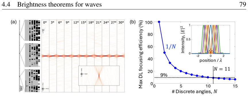
Figure 22. Figure 22: Metalens concentrator bounds. (a) A metalens concentrator that focuses 11 incoming-wave angles (incoherently) to a diffraction-limited (DL) spot [224]. (b) Bounds to maximum DL focusing efficiency for N incoherent excitations; the design of (a) has at most 9% DL focusing efficiency. (b, inset) The first five orthogonal-field-pattern intensities at the focusing plane, ordered from most to least concentrate… view at source ↗
Figure 23
Figure 23. Figure 23: Brightness theorem constraints in resonant TCMT. Incoherent excitations of a two-port waveguide (exemplified by a variable relative phase θ), cannot lead to resonance-assisted unity transmission with fewer than two output ports (a,e) or fewer than two resonance (b,f). (c,g) A design via coupled mode theory that achieves unity transmission. (d) A comparison of the three transmissions, as a function of phas… view at source ↗
Figure 24
Figure 24. Figure 24: Saturating the optical-theorem bounds with plasmonic and superscattering designs. (a) Plasmonic core–shell superscatterer [236]: TM channels of total angular momentum ℓ = 1,2,3 are tuned to a common frequency ω = 0.2932ωp, so the total scattering cross-section (blue) approaches 15λ 2/2π, well above any of the individual per-channel bounds (2ℓ+1)λ 2/2π of Eq. (153). (b) Per-volume absorption (blue) and sca… view at source ↗
Figure 25
Figure 25. Figure 25: Optical-theorem bounds across all size regimes. (a) Extinction cross-section bounds for an Ag scatterer enclosed in a spherical region of radius R, illuminated by a plane wave at λ = 360 nm. The general bound Eq. (158) (black) tracks the realized Ag-sphere cross-section (green) within a small factor over four decades in size. (b) Absorption, scattering, and extinction bounds for an arbitrary obstacle of r… view at source ↗
Figure 26
Figure 26. Figure 26: Tightened bounds via reactive-power constraint. With the addition of a reactive power constraint, one can tighten bounds (solid lines) for subwavelength dielectric scatterers, relative to optical-theorem-only constraints (dashed lines). (Figure adapted from Ref. [255].) conservation only (dashed lines) leads to absorption cross-section bounds that scale with scatterer volume (thereby increasing relative t… view at source ↗
Figure 27
Figure 27. Figure 27: Spectral response and sum rules in three prototypical scatterers. (a) A graphene sheet, (b) a TiO2 film, and (c) a silver sphere. (d) The extinction cross-section for a z-directed plane wave, normalized to the area/volume Ω, displays wide-ranging spectral behavior, yet always converges to the sum rule of Eq. (169). Conversely, one can take the high-frequency asymptotic limit of the KK relation, Eq. (165).… view at source ↗
Figure 28
Figure 28. Figure 28: Confirmation of the plasma-frequency-based sum rule for a dielectric material. (a) Simulated extinction cross-sections for a variety of antenna shapes and (b) their extinction as a function of total number of electrons. (c) Spectral contributions to extinction for a silicon sphere (top) and sphere dimer (bottom); notice the bump in extinction at energies above 100 eV, from core electrons that are counted … view at source ↗
Figure 29
Figure 29. Figure 29: LDOS sum rules from contour integration. (a) Schematic for LDOS calcula￾tion above a 2D sheet or 3D half-space, computed by a contour around the singularity at the origin (bottom). (b) Confirmation of the sum rule for 2D and 3D materials. The sum rules of these simply high-symmetry geometries also bound the all-frequency integrals for any scatterer contained within them, via monotonicity theorems. (Figure… view at source ↗
Figure 30
Figure 30. Figure 30: Common matrices constituting input–output relations in linear electro￾magnetism. For the first three, (a)–(c), it is an open question whether a KK relation, a sum rule, and a simple passivity condition can be combined for meaningful bounds. (d) Volume T matrices, which relate incident fields in a scatterer’s volume to the polarization fields they induce, exhibit all three in tandem, yielding the simple ca… view at source ↗
Figure 31
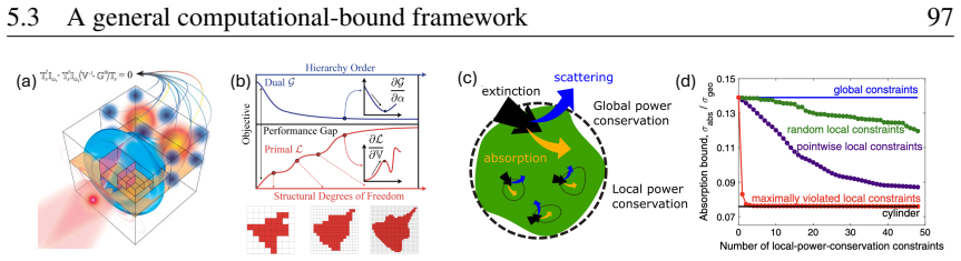
Figure 31. Figure 31: Computational bounds via local conservation laws. (a) The hierarchical mean-field T-operator viewpoint: a structured scatterer inside a designable cubic domain (light blue), partitioned into nested subdomains. Constraints on the scattering T operator are imposed on each subdomain rather than only globally. (b) As the hierarchy order increases (more, finer clusters), the convex dual bound tightens from abo… view at source ↗
Figure 32
Figure 32. Figure 32: Applications of the computational-bound framework. (a) Bounds on the near-field radiative Purcell enhancement of a dipole emitter coupled to a spherical, freeform￾patternable dielectric domain, plotted against the domain radius R/λ for several values of the material loss Imχ. Light curves apply only global conservation; dark curves apply the hierarchical local constraints and tighten the bounds by more th… view at source ↗
Figure 33
Figure 33. Figure 33: Multi-functional design via cross-correlation constraints. (Left) A multi￾functional device must produce distinct responses—different focal spots, scattering pat￾terns, transmission angles, etc.—across multiple incident fields, frequencies, or material configurations, while comprising a single physical structure. (Middle) Without cross￾correlation constraints, the bound formulation treats each scenario in… view at source ↗
Figure 34
Figure 34. Figure 34: Limits on the polarizability of small scatterers. Magnitude of the electric￾dipole polarizability for a representative small scatterer (a subwavelength sphere composed of a lossy Drude metal with ε/ε0 = ε∞ −ω 2 p/(ω 2 +iγmω) and ε∞ > 1), illustrating some of the limits discussed in Sections 5.4, 5.5. arbitrarily close, leading to a vanishing linewidth (corresponding to a complex-frequency pole of the pola… view at source ↗
Figure 35
Figure 35. Figure 35: Energy requirements for resonance in photonic and plasmonic structures. (a) In a conventional optical cavity with dimensions larger than approximately half a wavelength, the stored energy oscillates (indefinitely, in the lossless case) between electric￾field energy (left) and magnetic-field energy (right). (b) In a subwavelength dielectric cavity, the magnetic energy is too small to support a self-sustain… view at source ↗
Figure 36
Figure 36. Figure 36: Quality factor of plasmonic resonances in subwavelength metallic nanos￾tructures, as a function of resonance frequency, for gold (dashed line) and silver (dotted line). In the quasi-static regime, once the resonance frequency and the plasmonic material are specified, the Q-factor is uniquely determined and cannot be improved by structuring. (Figure adapted from Ref. [329].) electric field energy to the en… view at source ↗
Figure 37
Figure 37. Figure 37: Minimum mode volumes of 2D dielectric cavities. (a) For scalar waves (or vector waves with out-of-plane polarization), there can be no singular field response, and the minimum mode volume scales with λ 2 and cannot be further reduced by fine features of size d ≪ λ. (b) For vector waves (in-plane polarization), the mode volume can be decreased (at a fixed wavelength λ) with increasingly fine features. A ke… view at source ↗
Figure 38
Figure 38. Figure 38: Light confinement beyond the diffraction limit in all-dielectric structures. (a) Example of a structure supporting a strongly confined electric field distribution associ￾ated with a deeply subwavelength mode volume. The structure consists of a 3D biconical antenna embedded within a twisted photonic crystal cavity. Although the mode volume, as defined in Eq. (198), is subwavelength, the overall physical si… view at source ↗
Figure 39
Figure 39. Figure 39: Fundamental tradeoffs among scattering, absorption, and directivity. (a) Admissible values of the absorption-to-scattering ratio for a given absorption level, as dictated by passivity for spherically symmetric scatterers. The boundary of the blue shaded region represents the optimal scattering-absorption tradeoff achievable by passive objects. (b) Optimal tradeoff between absorption efficiency and antenna… view at source ↗
Figure 40
Figure 40. Figure 40: Perfect invisibility? Scattering cross sections, as a function of frequency, that are allowed and disallowed for finite, causal, stable scattering systems in free space. Nontrivial perfect invisibility is only possible on a discrete set of frequencies. scattering amplitude s(ω,0,φ) is analytic in the upper half of the complex-frequency plane, Imω > 0, as a consequence of causality and stability. We furthe… view at source ↗
Figure 41
Figure 41. Figure 41: A global bound on cloaking. Normalized scattering cross section over a broad wavelength range for different cloaking techniques. The cloaks are designed to suppress the scattering of (a) a dielectric sphere and (b) a perfectly conducting sphere at the central wavelength λc. In both panels, the scattering spectrum of the uncloaked object (black curve) is compared with those of several passive cloaks: a pla… view at source ↗
Figure 42
Figure 42. Figure 42: Fundamental bandwidth bounds on spherical-wave, plane-wave, and guided-wave reflection. Interpretation of Eqs. (210) (spherical-wave absorption), (213) (Rozanov bound), and (215) (Bode–Fano limit) as fundamental tradeoffs between in-band reflection magnitude and bandwidth. These tradeoffs are governed by physical size in Eqs. (210) and (213), and by the properties of the load impedance in Eq. (215). For a… view at source ↗
Figure 43
Figure 43. Figure 43: The impedance-matching problem. Circuit topology used in the derivation of the Bode-Fano limit on broadband impedance matching. in Eq. (209) for the spherical case, assuming |Γ(ω)| = 1 outside the finite bandwidth of interest, one obtains |lnΓ0|B π ≤ k0∑ i µs,idi , (213) where B = (λ2 −λ1)/λ0 is the fractional bandwidth around the center wavelength λ0 (see [PITH_FULL_IMAGE:figures/full_fig_p127_43.png] view at source ↗
Figure 44
Figure 44. Figure 44: Physical bounds on cloaking. (a) Normalized scattering cross section of an impenetrable sphere of radius a = λ0 (black curve) and of two cloaking devices, compared with the approximate physical bound from Ref. [371] (dashed red line). Existing bounds on cloaking are essentially limits on the size–bandwidth–performance product, showing that, as the maximum allowed in-band scattering is reduced, the maximum… view at source ↗
Figure 45
Figure 45. Figure 45: Sensing with scattering resonances. (a) Typical experimental reflectance spectra for a refractive index sensor with noise, before (black curve) and after (gray curve) a perturbation. (b) Dependence of the total normalized Q-factor (orange curve) and resonance amplitude A(λ0) (blue curve) on the ratio QR/QNR. (Figure adapted from Ref. [375].) derivative, in principle, diverges in the vicinity of the except… view at source ↗
Figure 46
Figure 46. Figure 46: Limits to the delay-bandwidth product. (a) Dispersion diagram of a guided mode with linear dispersion (red line, shown only within the bandwidth ∆ω) bounded by the light lines corresponding to the maximum and minimum available refractive indices (blue lines). This construction is used to derive the delay-bandwidth-product limit for waveguiding structures made of transparent dielectric materials, Eq. (224)… view at source ↗
Figure 47
Figure 47. Figure 47: Application of delay-bandwidth limits to meta-optics. (a) Delay-line model of a thin, dispersion-engineered achromatic metalens. (b) Comparison of published achro￾matic metalens designs against the derived (normalized) bandwidth limits, shown as a function of numerical aperture (NA) and for different levels of monochromatic aberrations (wavefront deformations). (c) Schematic of a spaceplate, which effecti… view at source ↗
Figure 48
Figure 48. Figure 48: Toward a universal framework for fundamental limits of light interactions with matter, organized as a three-tier hierarchy: bounds on complex applications, bounds on basic photonic and electromagnetic response, and bounds on the constitutive material parameters themselves. and vgx is the transverse group velocity (different assumptions about vgx can be made; see [396]). A comparison between this bound and… view at source ↗

discussion (0)

Sign in with ORCID, Apple, or X to comment. Anyone can read and Pith papers without signing in.

Reference graph

Works this paper leans on

37 extracted references · 37 canonical work pages

  1. [1]

    Beiträge zur theorie des mikroskops und der mikroskopischen wahrnehmung

    1E. Abbe, “Beiträge zur theorie des mikroskops und der mikroskopischen wahrnehmung”, Archiv für mikroskopische Anatomie9, 413–468 (1873) (cit. on p. 3). 2E. Yablonovitch, “Statistical ray optics”, Journal of the Optical Society of America72, 899–907 (1982) (cit. on p. 3). 3H. M. Nussenzveig,Causality and dispersion relations(Academic Press, New York, NY,

  2. [2]

    Conservation-law-based global bounds to quantum optimal control

    (cit. on pp. 5, 9, 16, 18, 88, 93, 122, 123, 129). 4H. Zhang, Z. Kuang, S. Puri, and O. D. Miller, “Conservation-law-based global bounds to quantum optimal control”, Physical Review Letters127, 110506 (2021) (cit. on pp. 5, 97). 5W. Shockley and H. J. Queisser, “Detailed balance limit of efficiency of p-n junction solar cells”, J. Appl. Phys.32, 510–519 (...

  3. [3]

    A perfectly matched layer for the absorption of electromagnetic waves

    (cit. on p. 5). 11J.-P. Berenger, “A perfectly matched layer for the absorption of electromagnetic waves”, en, J. Comput. Phys.114, 185–200 (1994) (cit. on p. 7). 12Z. S. Sacks, D. M. Kingsland, R. Lee, and J.-F. Lee, “A perfectly matched anisotropic absorber for use as an absorbing boundary condition”, IEEE Trans. Antennas Propag. 43, 1460–1463 (1995) (c...

  4. [4]

    Perfect single-sided radiation and absorption without mirrors

    (cit. on p. 9). Bibliography 142 18H. Zhou, B. Zhen, C. W. Hsu, O. D. Miller, S. G. Johnson, J. D. Joannopoulos, and M. Soljaˇci´c, “Perfect single-sided radiation and absorption without mirrors”, Optica3, 1079–1086 (2016) (cit. on p. 10). 19M. Yildirim, N. U. Dinç, I. Oguz, D. Psaltis, and C. Moser, “Nonlinear processing with linear optics”, Nat. Photoni...

  5. [5]

    Time-varying media, dispersion, and the princi- ple of causality

    (cit. on pp. 10, 11, 13, 83). 22T. T. Koutserimpas and F. Monticone, “Time-varying media, dispersion, and the princi- ple of causality”, Optical Materials Express14, 1222–1236 (2024) (cit. on pp. 12, 28, 41). 23J. Pendry, “Photon number conservation in time dependent systems”, Optics Express 31, 452–458 (2022) (cit. on p. 12). 24Z. Hayran and F. Monticone...

  6. [6]

    Complex-frequency excitations in photonics and wave physics

    (cit. on pp. 14, 24, 25, 29, 30, 50, 86, 129). 36S. Kim, A. Krasnok, and A. Alù, “Complex-frequency excitations in photonics and wave physics”, Science387, eado4128 (2025) (cit. on p. 14). 37H. A. Haus,Waves and fields in optoelectronics(Prentice-Hall,

  7. [7]

    Electro- magnetic nonreciprocity

    (cit. on pp. 14, 15, 118, 133). 39C. Caloz, A. Alu, S. Tretyakov, D. Sounas, K. Achouri, and Z.-L. Deck-Léger, “Electro- magnetic nonreciprocity”, Physical Review Applied10, 047001 (2018) (cit. on pp. 14, 15). 40D. Jalas, A. Petrov, M. Eich, W. Freude, S. Fan, Z. Yu, R. Baets, M. Popovi´c, A. Melloni, J. D. Joannopoulos, et al., “What is—and what is not—a...

  8. [8]

    Broadband and giant nonreciprocity at the subwavelength scale in magnetoplasmonic materials

    (cit. on pp. 17, 19, 30, 37, 40, 89, 90, 105, 121). 46M. I. Abdelrahman and F. Monticone, “Broadband and giant nonreciprocity at the subwavelength scale in magnetoplasmonic materials”, Physical Review B102, 155420 (2020) (cit. on p. 17). 47R. M. Foster, “A reactance theorem”, Bell System technical journal3, 259–267 (1924) (cit. on p. 18). 48P. Triverio, S...

  9. [9]

    Causality and passivity: from electromagnetism and network theory to metamaterials

    (cit. on p. 18). 50A. Srivastava, “Causality and passivity: from electromagnetism and network theory to metamaterials”, Mechanics of Materials154, 103710 (2021) (cit. on p. 18). Bibliography 144 51D. Youla, L. Castriota, and H. Carlin, “Bounded real scattering matrices and the founda- tions of linear passive network theory”, IRE Transactions on Circuit Th...

  10. [10]

    Physical limitations on broadband invisibility based on fast-light media

    (cit. on pp. 18, 19, 28, 30, 32, 40, 41, 120, 126). 55M. I. Abdelrahman, Z. Hayran, A. Chen, and F. Monticone, “Physical limitations on broadband invisibility based on fast-light media”, Nature Communications12, 3041 (2021) (cit. on p. 19). 56G. Raisbeck, “A definition of passive linear networks in terms of time and energy”, Journal of Applied Physics25, ...

  11. [11]

    Dissipative dynamical systems part ii: linear systems with quadratic supply rates

    (cit. on pp. 19, 20). 59J. C. Willems, “Dissipative dynamical systems part ii: linear systems with quadratic supply rates”, Archive for rational mechanics and analysis45, 352–393 (1972) (cit. on p. 19). 60S. Boyd and L. O. Chua, “On the passivity criterion for lti n-ports”, International Journal of Circuit Theory and Applications10, 323–333 (1982) (cit. o...

  12. [12]

    Nonlocal response in plasmonic nanostructures

    (cit. on p. 28). 80M. Wubs and N. A. Mortensen, “Nonlocal response in plasmonic nanostructures”, in Quantum plasmonics(Springer, 2016), pp. 279–302 (cit. on p. 28). 81R. W. Boyd,Nonlinear optics(Academic Press,

  13. [13]

    Energy of electromagnetic waves in the presence of absorption and dispersion

    (cit. on pp. 29, 102, 103). 83J. Askne and B. Lind, “Energy of electromagnetic waves in the presence of absorption and dispersion”, Physical Review A2, 2335 (1970) (cit. on pp. 30, 111). 84S. A. Ramakrishna and T. M. Grzegorczyk,Physics and applications of negative refractive index materials(CRC press,

  14. [14]

    Linear and nonlinear wave propagation in negative refraction metamaterials

    (cit. on pp. 30, 111). Bibliography 146 85V . Agranovich, Y . Shen, R. H. Baughman, and A. A. Zakhidov, “Linear and nonlinear wave propagation in negative refraction metamaterials”, Physical Review B69, 165112 (2004) (cit. on p. 30). 86M. G. Silveirinha, “Metamaterial homogenization approach with application to the characterization of microstructured comp...

  15. [15]

    Fundamental limits to the refractive index of transparent optical materials

    (cit. on pp. 31, 48, 104, 112, 113). 88H. Shim, F. Monticone, and O. D. Miller, “Fundamental limits to the refractive index of transparent optical materials”, Advanced Materials33, 2103946 (2021) (cit. on pp. 31, 33–35). 89L. Zhang, F. Monticone, and O. D. Miller, “All electromagnetic scattering bodies are matrix-valued oscillators”, Nature Communications...

  16. [16]

    Maximum refractive index of an atomic medium

    (cit. on p. 32). 91C. Caloz,Physical interpretation of a simple sum rule, Private communication, 2019 (cit. on p. 32). 92F. Andreoli, M. J. Gullans, A. A. High, A. Browaeys, and D. E. Chang, “Maximum refractive index of an atomic medium”, Physical Review X11, 011026 (2021) (cit. on p. 34). 93F. Andreoli, B. Windt, S. Grava, G. M. Andolina, M. J. Gullans, ...

  17. [17]

    The uniqueness theorem for nonlocal hydrodynamic media

    (cit. on p. 37). Bibliography 147 101C. Mystilidis, G. Fikioris, C. Tserkezis, G. A. Vandenbosch, and X. Zheng, “The uniqueness theorem for nonlocal hydrodynamic media”, IEEE Transactions on Antennas and Propagation (2024) (cit. on p. 37). 102A. Ishimaru,Electromagnetic wave propagation, radiation, and scattering: from funda- mentals to applications(John ...

  18. [18]

    Nonreciprocal cavities and the time–bandwidth limit

    (cit. on p. 38). 103S. A. Mann, D. L. Sounas, and A. Alu, “Nonreciprocal cavities and the time–bandwidth limit”, Optica6, 104–110 (2019) (cit. on pp. 38, 135). 104D. E. Fernandes and M. G. Silveirinha, “Topological origin of electromagnetic energy sinks”, Physical Review Applied12, 014021 (2019) (cit. on p. 38). 105J. D. Dow and D. Redfield, “Toward a uni...

  19. [19]

    How to deal with the loss in plasmonics and metamaterials

    (cit. on p. 39). 107J. B. Khurgin, “How to deal with the loss in plasmonics and metamaterials”, Nature nanotechnology10, 2–6 (2015) (cit. on pp. 39, 108, 109). 108S. A. Hassani Gangaraj and F. Monticone, “Physical violations of the bulk-edge corre- spondence in topological electromagnetics”, Physical review letters124, 153901 (2020) (cit. on p. 39). 109X....

  20. [20]

    Physical limits on electronic nonlinear molecular susceptibilities

    (cit. on p. 41). Bibliography 148 118M. G. Kuzyk, “Physical limits on electronic nonlinear molecular susceptibilities”, Physical review letters85, 1218 (2000) (cit. on pp. 41, 42). 119M. G. Kuzyk, “Erratum: physical limits on electronic nonlinear molecular suscepti- bilities [phys. rev. lett. 85, 001218 (2000)]”, Physical Review Letters90, 1218 (2003) (ci...

  21. [21]

    Radiating and nonradiating classical current distributions and the fields they generate

    (cit. on p. 50). 137A. J. Devaney and E. Wolf, “Radiating and nonradiating classical current distributions and the fields they generate”, Phys. Rev. D8, 1044–1047 (1973) (cit. on p. 51). 138S. W. Hell and J. Wichmann, “Breaking the diffraction resolution limit by stimulated emission: stimulated-emission-depletion fluorescence microscopy”, Opt. Lett.19, 78...

  22. [22]

    Inverse design in nanophotonics

    (cit. on p. 55). 160S. Molesky, Z. Lin, A. Y . Piggott, W. Jin, J. Vuckovi´c, and A. W. Rodriguez, “Inverse design in nanophotonics”, en, Nat. Photonics12, 659–670 (2018) (cit. on p. 55). 161 ˇC. Brukner and A. Zeilinger, “Diffraction of matter waves in space and in time”, Phys. Rev. A56, 3804–3824 (1997) (cit. on p. 55). 162A. Goussev, “Diffraction in ti...

  23. [23]

    Chester, Second sound in solids, Phys

    (cit. on pp. 59, 100). 168W. J. Welch, “Reciprocity theorems for electromagnetic fields whose time-dependence is arbitrary”, IRE Trans. Antennas Propag.8, 68–73 (1960) (cit. on p. 60). 169A. T. de Hoop, “Time-domain reciprocity theorems for electromagnetic fields in disper- sive media”, Radio Sci.22, 1171–1178 (1987) (cit. on p. 60). Bibliography 151 170B...

  24. [24]

    Communicating with waves between volumes: evaluating orthogonal spatial channels and limits on coupling strengths

    (cit. on p. 64). 191D. A. Miller, “Communicating with waves between volumes: evaluating orthogonal spatial channels and limits on coupling strengths”, Applied optics39, 1681–1699 (2000) (cit. on pp. 64, 65). 192D. A. B. Miller, L. Zhu, and S. Fan, “Universal modal radiation laws for all thermal emitters”, Proc. Natl. Acad. Sci. U. S. A.114, 4336–4341 (201...

  25. [25]

    Nonimaging optics: a tutorial

    (cit. on pp. 76, 78). 212R. Winston, L. Jiang, and M. Ricketts, “Nonimaging optics: a tutorial”, Adv. Opt. Photonics (2018) (cit. on p. 76). 213H. Goldstein, C. P. Poole, J. Safko, et al.,Classical mechanics, V ol. 2 (Addison-wesley Reading, MA,

  26. [26]

    Observation of parity–time symmetry in optics

    (cit. on p. 76). 214C. E. Rüter, K. G. Makris, R. El-Ganainy, D. N. Christodoulides, M. Segev, and D. Kip, “Observation of parity–time symmetry in optics”, en, Nat. Phys.6, 192–195 (2010) (cit. on p. 77). 215A. Regensburger, C. Bersch, M.-A. Miri, G. Onishchukov, D. N. Christodoulides, and U. Peschel, “Parity-time synthetic photonic lattices”, en, Nature4...

  27. [27]

    Coherency matrix formulation for partially coherent imaging to evaluate the degree of coherence for image

    (cit. on p. 78). 220K. Yamazoe, “Coherency matrix formulation for partially coherent imaging to evaluate the degree of coherence for image”, J. Opt. Soc. Am. A29, 1529 (2012) (cit. on p. 78). 221C. Okoro, H. E. Kondakci, A. F. Abouraddy, and K. C. Toussaint, “Demonstration of an optical-coherence converter”, Optica4, 1052 (2017) (cit. on p. 78). 222E. Wol...

  28. [28]

    Topology optimization of freeform large-area metasurfaces

    (cit. on p. 79). 224Z. Lin, V . Liu, R. Pestourie, and S. G. Johnson, “Topology optimization of freeform large-area metasurfaces”, Opt. Express27, 15765–15775 (2019) (cit. on p. 79). 225W. Suh, Z. Wang, and S. Fan, “Temporal coupled-mode theory and the presence of non-orthogonal modes in lossless multimode cavities”, IEEE J. Quantum Electron.40, 1511–1518...

  29. [29]

    Fundamental limits to optical response in absorptive systems

    (cit. on pp. 80, 135). 227O. D. Miller, A. G. Polimeridis, M. T. H. Reid, C. W. Hsu, B. G. DeLacy, J. D. Joannopoulos, M. Soljaˇci´c, and S. G. Johnson, “Fundamental limits to optical response in absorptive systems”, Opt. Express24, 3329 (2016) (cit. on pp. 81, 84). 228Y . Yang, O. D. Miller, T. Christensen, J. D. Joannopoulos, and M. Soljaˇci´c, “Low-los...

  30. [30]

    Optimal characteristics of an arbitrary receive antenna

    (cit. on p. 82). 233D.-H. Kwon and D. M. Pozar, “Optimal characteristics of an arbitrary receive antenna”, IEEE Trans. Antennas Propag.57, 3720–3727 (2009) (cit. on pp. 82, 83). 234Z. Kuang, L. Zhang, and O. D. Miller, “Maximal single-frequency electromagnetic response”, Optica7, 1746–1757 (2020) (cit. on pp. 82, 83, 85, 86). Bibliography 155 235Z. Ruan a...

  31. [31]

    Upper bounds on focusing efficiency

    (cit. on pp. 85, 140). 241M. Gustafsson, K. Schab, L. Jelinek, and M. Capek, “Upper bounds on focusing efficiency”, Optics Express30, 46490–46508 (2022) (cit. on p. 85). 242Y . Ivanenko, M. Gustafsson, and S. Nordebo, “Optical theorems and physical bounds on absorption in lossy media”, Optics Express27, 34323–34342 (2019) (cit. on p. 86). 243O. D. Miller,...

  32. [32]

    On the passivity criterion for ltiN-ports

    (cit. on p. 93). 280S. Boyd and L. O. Chua, “On the passivity criterion for ltiN-ports”, en, Int. J. Circuit Theory Appl.10, 323–333 (1982) (cit. on p. 93). 281A. Bernland, A. Luger, and M. Gustafsson, “Sum rules and constraints on passive systems”, en, J. Phys. A: Math. Theor.44, 145205 (2011) (cit. on p. 93). 282A. Srivastava, “Causality and passivity: ...

  33. [33]

    All electromagnetic scattering bodies are matrix-valued oscillators

    (cit. on p. 94). 288L. Zhang, F. Monticone, and O. Miller, “All electromagnetic scattering bodies are matrix-valued oscillators”, Nat. Commun.14, 10.1038/s41467-023-43221-2 (2023) (cit. on pp. 94, 95). 289Z. Kuang and O. D. Miller, “Computational bounds to light–matter interactions via local conservation laws”, Phys. Rev. Lett.125, 263607 (2020) (cit. on ...

  34. [34]

    An optimal-storage approach to semidefinite programming using approximate complementarity

    (cit. on p. 97). 294L. Ding, A. Yurtsever, V . Cevher, J. A. Tropp, and M. Udell, “An optimal-storage approach to semidefinite programming using approximate complementarity”, en, SIAM J. Optim.31, 2695–2725 (2021) (cit. on p. 97). 295K. Anstreicher and H. Wolkowicz, “On lagrangian relaxation of quadratic matrix constraints”, SIAM J. Matrix Anal. Appl.22, ...

  35. [35]

    Embedded photonic eigenvalues in 3d nanostructures

    (cit. on pp. 104, 108). 304F. Monticone and A. Alu, “Embedded photonic eigenvalues in 3d nanostructures”, Physical Review Letters112, 213903 (2014) (cit. on pp. 104, 106, 107). 305D. Jones, “Scattering by inhomogeneous dielectric particles”, The Quarterly Journal of Mechanics and Applied Mathematics38, 135–155 (1985) (cit. on pp. 105, 121). 306D. Sjöberg,...

  36. [36]

    Theoretical limitations on the broadband matching of arbitrary impedances

    (cit. on p. 127). 366R. M. Fano, “Theoretical limitations on the broadband matching of arbitrary impedances”, Journal of the Franklin Institute249, 57–83 (1950) (cit. on pp. 127, 128). 367H. Carlin and P. Civalleri, “Wideband circuit design, ser”, Electronic Engineering Systems Series. Boca Raton, Fla: CRC Press (1998) (cit. on p. 127). 368D. Nie and B. M...

  37. [37]

    Compact all-pass filters in photonic crystals as the building block for high-capacity optical delay lines

    (cit. on pp. 134, 137). 389Z. Wang and S. Fan, “Compact all-pass filters in photonic crystals as the building block for high-capacity optical delay lines”, Physical Review E68, 066616 (2003) (cit. on p. 135). 390S. A. Hassani Gangaraj and F. Monticone, “Do truly unidirectional surface plasmon- polaritons exist?”, Optica6, 1158–1165 (2019) (cit. on p. 135)...

This paper was first reviewed by grok-4.3 on June 30, 2026.